Artificial Intelligence and Machine Learning: Unit V: Neural Networks
Regularization
Neural Networks - Artificial Intelligence and Machine Learning
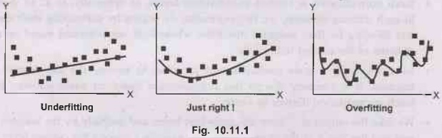
Just have a look at the above figure, and we can immediately predict that once we try to cover every minutest feature of the input data, there can be irregularities in the extracted features, which can introduce noise in the output. This is referred to as "Overfitting".
Regularization
•
Just have a look at the above figure, and we can
immediately predict that once we try to cover every minutest feature of the
input data, there can be irregularities in the extracted features, which can
introduce noise in the output. This is referred to as "Overfitting".
•
This may also happen with the lesser number of
features extracted as some of the important details might be missed out. This
will leave an effect on the accuracy of the outputs produced. This is referred
to as "Underfitting".
•
This also shows that the complexity for processing
the input elements increases with overfitting. Also, neural networks being a
complex interconnection of nodes, the issue of overfitting may arise
frequently.
•
To eliminate this, regularization is used, in which
we have to make the slightest modification in the design of the neural network,
and we can get better outcomes.
Regularization in Machine Learning
•
One of the most important factors that affect the
machine learning model is overfitting.
•
The machine learning model may perform poorly if it
tries to capture even the noise present in the dataset applied for training the
system, which ultimately results in overfitting. In this context, noise doesn't
mean the ambiguous or false data, but those inputs which do not acquire the
required features to execute the machine learning model.
•
Analyzing these data inputs may surely make the model
flexible, but the risk of overfitting will also increase accordingly.
•
One of the ways to avoid this is to cross validate
the training dataset, and decide accordingly the parameters to include that can
increase the efficiency and performance of the model.
•
Let this be the simple relation for linear regression
Where
Y =
b0 + b1X1 + b2X2 + ....
bpXp
Y =
Learned relation
B =
Co-efficient estimators for different variables and/or predictors (X)
•
Now, we shall introduce a loss function, that
implements the fitting procedure, which is referred to as "Residual Sum of
Squares" or RSS.
•
The co-efficient in the function is chosen in such a
way that it can minimize the loss function easily.
Hence,
RSS =
Σni=1 (Υi – β0 – Σpj=1
βi Χij )2
•
Above equation will help in adjusting the
co-efficient function depending on the training dataset.
•
In case noise is present in the training dataset,
then the adjusted co-efficient won't be generalized when the future datasets
will be introduced. Hence, at this point, regularization comes into picture and
makes this adjusted co-efficient shrink towards zero.
•
One of the methods to implement this is the ridge
regression, also known as L2 regularization. Lets have a quick overview on
this.
Ridge Regression (L2 Regularization)
•
Ridge regression, also known as L2 regularization, is
a technique of regularization to avoid the overfitting in training data set,
which introduces a small bias in the Straining model, through which one can get
long term predictions for that input.
•
In this method, a penalty term is added to the cost
function. This amount of bias altered to the cost function in the model is also
known as ridge regression penalty.
•
Hence, the equation for the cost function, after
introducing the ridge regression penalty is as follows:
Σmi=1
(yi – y`i)2 = Σni=1 (Υi
– Σnj=1 βj × Χij)2 + λ Σnj=0
βj2
Here,
λ is multiplied by the square of the weight set for the individual feature of
the input data. This term is ridge regression penalty.
•
It regularizes the co-efficient set for the model and
hence the ridge regression term deduces the values of the coefficient, which
ultimately helps in deducing the complexity of the machine learning model.
•
From the above equation, we can observe that if the
value of tends to zero, the last term on the right hand side will tend to zero,
thus making the above equation a representation of a simple linear regression
model.
•
Hence, lower the value of, the model will tend to
linear regression.
•
This model is important to execute the neural
networks for machine learning, as there would be risks of failure for
generalized linear regression models, if there are dependencies found between
its variables. Hence, ridge regression is used here.
Lasso Regression (L1 Regularization)
•
One more technique to reduce the overfitting, and
thus the complexity of the model is the lasso regression.
•
Lasso regression stands for Least Absolute and
Selection Operator and is also sometimes known as L1 regularization.
•
The equation for the lasso regression is almost same
as that of the ridge regression, except for a change that the value of the
penalty term is taken as the absolute weights.
•
The advantage of taking the absolute values is that
its slope can shrink to 0, as compared to the ridge regression, where the slope
will shrink it near to 0.
•
The following equation gives the cost function
defined in the Lasso regression:
Σmi=1
(yi – y`i)2 = Σni=1 (Υi
– Σni=1 βj × Χij) + λ Σni=0
| βj|2
•
Due to the acceptance of absolute values for the cost
function, some of the features of the input dataset can be ignored completely
while evaluating the machine learning model, and hence the feature selection
and overfitting can be reduced to much extent.
•
On the other hand, ridge regression does not ignore
any feature in the model and includes it all for model evaluation. The
complexity of the model can be reduced using the shrinking of co-efficient in
the ridge regression model.
Dropout
•
Dropout was introduced by "Hinton et al"and
this method is now very popular. It consists of setting to zero the output of
each hidden neuron in chosen layer with some probability and is proven to be
very effective in reducing overfitting.
•
Fig. 10.11.2 shows dropout regulations.
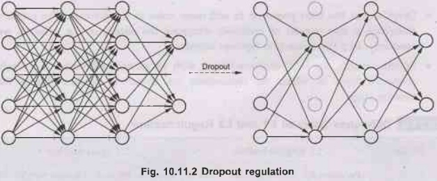
•
To achieve dropout regularization, some neurons in
the artificial neural network are randomly disabled. That prevents them from
being too dependent on one another as they learn the correlations. Thus, the
neurons work more independently, and the artificial neural network learns
multiple independent correlations in the data based on different configurations
of the neurons.
•
It is used to improve the training of neural networks
by omitting a hidden unit. It also speeds training.
•
Dropout is driven by randomly dropping a neuron so
that it will not contribute to the forward pass and back-propagation.
•
Dropout is an inexpensive but powerful method of
regularizing a broad family of es models.
DropConnect
•
DropConnect, known as the generalized
version of Dropout, is the method used brts for regularizing deep neural
networks. Fig. 10.11.3 shows dropconnect.
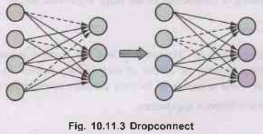
•
DropConnect has been proposed to add more noise to
the network. The primary difference is that instead of randomly dropping the
output of the neurons, we randomly drop the connection between neurons.
•
In other words, the fully connected layer with
DropConnect becomes a sparsely connected layer in which the connections are
chosen at random during the training stage.
Difference between L1 and L2 Regularization

Artificial Intelligence and Machine Learning: Unit V: Neural Networks : Tag: : Neural Networks - Artificial Intelligence and Machine Learning - Regularization
Related Topics
Related Subjects

Artificial Intelligence and Machine Learning
CS3491 4th Semester CSE/ECE Dept | 2021 Regulation | 4th Semester CSE/ECE Dept 2021 Regulation