Regression

Regression

• For an input x, if the output is continuous, this is called a regression problem. For example, based on historical information of demand for tooth paste in your supermarket, you are asked to predict the demand for the next month.

• Regression is concerned with the prediction of continuous quantities. Linear regression is the oldest and most widely used predictive model in the field of machine learning. The goal is to minimize the sum of the squared errors to fit a straight line to a set of data points.

• It is one of the supervised learning algorithms. A regression model requires the knowledge of both the dependent and the independent variables in the training data set.

• Simple Linear Regression (SLR) is a statistical model in which there is only one independent variable and the functional relationship between the dependent variable and the regression coefficient is linear.

• Regression line is the line which gives the best estimate of one variable from the value of any other given variable.

• The regression line gives the average relationship between the two variables in mathematical form. For two variables X and Y, there are always two lines of regression.

• Regression line of Y on X: Gives the best estimate for the value of Y for any specific given values of X:

where

Y = a + bx

a = Y - intercept

b = Slope of the line

Y = Dependent variable

X = Independent variable

• By using the least squares method, we are able to construct a best fitting straight line to the scatter diagram points and then formulate a regression equation in the form of:

ŷ = a + bx

ŷ = ȳ + b(x- x̄)      

• Regression analysis is the art and science of fitting straight lines to patterns of data. In a linear regression model, the variable of interest ("dependent" variable) is predicted from k other variables ("independent" variables) using a linear equation.

• If Y denotes the dependent variable and X₁, ..., X_k are the independent variables, then the assumption is that the value of Y at time t in the data sample is determined by the linear equation:

Y₁ = β₀ + β₁ X_1t + B₂ X_2t +… + β_k X_kt + ε_t

where the betas are constants and the epsilons are independent and identically distributed normal random variables with mean zero.

Regression Line

• A way of making a somewhat precise prediction based upon the relationships between two variables. The regression line is placed so that it minimizes the predictive error.

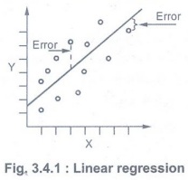
• The regression line does not go through every point; instead it balances the difference between all data points and the straight-line model. The difference between the observed data value and the predicted value (the value on the straight line) is the error or residual. The criterion to determine the line that best describes the relation between two variables is based on the residuals.

Residual = Observed - Predicted

• A negative residual indicates that the model is over-predicting. A positive residual indicates that the model is under-predicting.

Linear Regression

• The simplest form of regression to visualize is linear regression with a single predictor. A linear regression technique can be used if the relationship between X and Y can be approximated with a straight line.

• Linear regression with a single predictor can be expressed with the equation:

              y = Ɵ₂x + Ɵ₁ + e

• The regression parameters in simple linear regression are the slope of the line (Ɵ₂), the angle between a data point and the regression line and the y intercept (Ɵ₁) the point where x crosses the y axis (X = 0).

• Model 'Y', is a linear function of 'X'. The value of 'Y' increases or decreases in linear manner according to which the value of 'X' also changes.

Nonlinear Regression:

• Often the relationship between x and y cannot be approximated with a straight line. In this case, a nonlinear regression technique may be used.

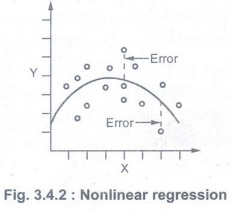
• Alternatively, the data could be preprocessed to make the relationship linear. In Fig. 3.4.2 shows nonlinear regression. (Refer Fig. 3.4.2 on previous page)

• The X and Y have a nonlinear relationship.sp

• If data does not show a linear dependence we can get a more accurate model using a nonlinear regression model.

• For example: y = W₀ + W₁X + W₂ X² + W₃ X³

• Generalized linear model is foundation on which linear regression can be applied to modeling categorical response variables.

Advantages:

a. Training a linear regression model is usually much faster than methods such as neural networks.

b. Linear regression models are simple and require minimum memory to implement.

c. By examining the magnitude and sign of the regression coefficients you can infer how predictor variables affect the target outcome.

• There are two important shortcomings of linear regression:

1. Predictive ability: The linear regression fit often has low bias but high variance. Recall that expected test error is a combination of these two quantities. Prediction accuracy can sometimes be improved by sacrificing some small amount of bias in order to decrease the variance.

2. Interpretative ability: Linear regression freely assigns a coefficient to each predictor variable. When the number of variables p is large, we may sometimes seek, for the sake of interpretation, a smaller set of important variables.

Least Squares Regression Line

Least square method

• The method of least squares is about estimating parameters by minimizing the squared discrepancies between observed data, on the one hand and their expected values on the other.

• The Least Squares (LS) criterion states that the sum of the squares of errors is minimum. The least-squares solutions yield y(x) whose elements sum to 1, but do not ensure the outputs to be in the range [0, 1].

• How to draw such a line based on data points observed? Suppose a imaginary line of y = a + bx.

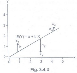
• Imagine a vertical distance between the line and a data point E = Y - E(Y). This error is the deviation of the data point from the imaginary line, regression line. Then what is the best values of a and b? A and b that minimizes the sum of such errors.

• Deviation does not have good properties for computation. Then why do we use squares of deviation? Let us get a and b that can minimize the sum of squared deviations rather than the sum of deviations. This method is called least squares.

• Least squares method minimizes the sum of squares of errors. Such a and b are called least squares estimators i.e. estimators of parameters a and B.

• The process of getting parameter estimators (e.g., a and b) is called estimation. Lest squares method is the estimation method of Ordinary Least Squares (OLS).

Disadvantages of least square

1. Lack robustness to outliers.

2. Certain datasets unsuitable for least squares classification.

3. Decision boundary corresponds to ML solution.

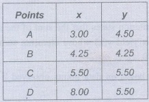
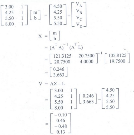
Example 3.4.1: Fit a straight line to the points in the table. Compute m and b by least squares.

Standard Error of Estimate

• The standard error of estimate represents a special kind of standard deviation that reflects tells that we the magnitude of predictive error. The standard error of estimate, denoted S approximately how large the prediction errors (residuals) are for our data set in the same units as Y.

Definition formula for standard error of estimate = √Sum of square / √n-2

Definition formula for standard error of estimate  = √Y-Y' / √(n-2)

Computation formula for standard error of estimate: S_y/x = √SS_y(1-r²) /n-2

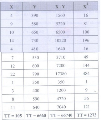
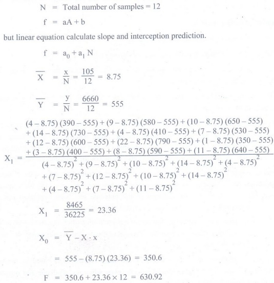
Example 3.4.2: Define linear and nonlinear regression using figures. Calculate the value of Y for X = 100 based on linear regression prediction method.

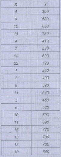
Solution