Searching Techniques

UNIT I

Chapter 4: Heuristic Search Strategies - Local Search and Optimization Problems

Searching Techniques

Introduction to Informed Search

• In the previous chapter 3 we have seen the concept of uninformed or blind search strategy. Now we will see more efficient search strategy, the informed search strategy. Informed search strategy is the search strategy that uses problem-specific knowledge beyond the definition of the problem itself.

• The general, method followed in informed search is best first search. Best first search is similar to graph search or tree search algorithm wherein node expansion is done based on certain criteria.

Generate-and-Test

• Generate-and-Test is a search algorithm which uses depth first search technique. It assures to find solution in systematic way. It generates complete solution and then the testing is done. A heuristic is needed so that the search is improved.

Following is the algorithm for Generate-and-Test :

1) Generate a possible solution which can either be a point in the problem space or a path from the initial state.

2) Test to see if this possible solution is a real (actual) solution by comparing the state reached with the set of goal states.

3) If it is real solution then return the solution otherwise repeat from state 1.

Following diagram illustrates the algorithm steps:

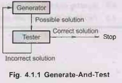
• Generate-and-Test is acceptable for simple problems whereas it is inefficient for problems with large spaces.

Best First Search Technique (BFS)

1) Search will start at root node.

2) The node to be expanded next is selected on the basis of an evaluation function, f(n).

3) The node having lowest value for f(n) is selected first. This lowest value of f(n) indicates that goal is nearest from this node (that is f(n) indicates distance from current node to goal node).

Implementation: BFS can be implemented using priority queue where fringe will be stored. The nodes in fringe will be stored in priority queue with increasing value of f(n) i.e. ascending order of f(n). The high priority will be given to node which has low f(n) value.

As name says "best first" then, we would always expect to have optimal solution. But in general BFS indicates that choose the node that appears to be best according to the evaluation function. Hence the optimality based on 'best-ness' of evaluation function.

Algorithm for best first search

1. Use two ordered lists OPEN and CLOSED.

2. Start with the initial node 'n' and put it on the ordered list OPEN.

3. Create a list CLOSED. This is initially an empty list.

4. If OPEN is empty then exit with failure.

5. Select first node on OPEN. Remove it from OPEN and put it on CLOSED. Call this node n.

6. If 'n' is the goal node exit. The solution is obtained by tracing a path backward along the arcs in the tree from 'n' to 'n1'.

7. Expand node 'n'. This will generate successors. Let the set of successors generated, be S. Create arcs from 'n' to each member of S.

8. Reorder the list OPEN, according to the heuristic and go back to step 4.

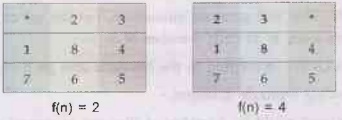
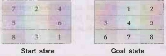
Consider the following 8-puzzle problem-

Here the heuristic used could be "number of tiles not in correct position" (i.e. number of tiles misplaced). In this solution the convention used is, that smaller value of the heuristic function 'f' leads earlier to the goal state.

Step 1

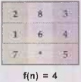
This is the initial state where four tiles (1, 2, 6, 8) are misplaced so value of heuristic function at this node is 4.

Step 2

This will be the next step of the tree.

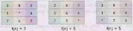
Heuristic function gives the values as 3, 5 and 5 respectively.

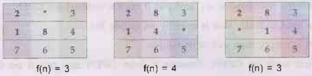
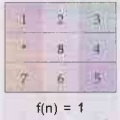
Step 3

Next, the node with the lowest f(n) value 3 is the one to be further expanded which generates 3 nodes.

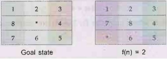
Step 4

Here there is tie for f(n) value. We continue to expand node.

Step 5

Step 6

In this algorithm a depth factor g is also added to h.

Heuristic Function

There are many different algorithms which employ the concept of best first search. The main difference between all the algorithms is that they have different evaluation function. The central component of these algorithms is heuristic function - h(n) which is defined as, h(n) = estimate cost of the cheapest path from node 'n' to a goal node.

Note

1) Heuristic function is key component of best first search. It is denoted by h(n) and h(n) = The shortest and cheapest path from initial node to goal node.

2) One can give additional knowledge about the problem to the heuristic function. For example - In our problem of Pune-Chennai route we can give information about distances between cities to the heuristic function.

3) A heuristic function guide the search in an efficient way.

4) A heuristic function h(n) consider a node as input but it rely only on the state at that node.

5) h(n) = 0, if n is goal state.

Greedy Best First Search (GBFS)

• Greedy best first search expand the node that is closest to the goal, expecting to get solution quickly:

• It evaluates node by using the heuristic function f(n) = h(n).

• It is termed as greedy (asking for more) because at each step it tries to get as close to the goal as it can.

• GBFS resembles DFS in the way that it prefers to follow a single path all the way to the goal. It back tracks when it comes to dead end that is, to a node from which goal state cannot be reached.

• Choosing minimum h(n) can lead to bad start as it may not yield always a solution. Also as this exploration is not leading to solution, therefore unwanted nodes are getting expanded.

• In GBFS, if repeated states are not detected then the solution will never found.

Performance measurement

1) Completeness: It is incomplete as it can start down an infinite path and never return to try other possibilities which can give solution.

2) Optimal: It is not optimal as it can initially select low value h(n) node but it may happen that some greater value node in current fringe can lead to better solution. Greedy strategies, in general, suffers from this, "looking for current best they loose on future best and inturn finally the best solution" !

3) Time and space complexity: Worst case time and space complexity is 0 (b^m) where 'm' is the maximum depth of the search space.

The complexity can be reduced by devicing good heuristic function.

A* Search

The A* algorithm

1) A* is most popular form of best first search.

2) A* evaluates node based on two functions namely

1) g(n) - The cost to reach the node 'n'.

2) h(n) - The cost to reach the goal node from node 'n'.

These two function's costs are combined into one, to evaluate a node. New function f(n) is deviced as,

f(n)=g(n) + h(n) that is,

f(n) = Estimated cost of the cheapest solution through 'n'.

Working of A*

1) The algorithm maintains two sets.

a) OPEN list: The OPEN list keeps track of those nodes that need to be examined.

b) CLOSED list: The CLOSED list keeps track of nodes that have already been examined.

2) Initially, the OPEN list contains just the initial node, and the CLOSED list is empty. Each node n maintains the following: g(n), h(1 h(n), f(n) as described above.

3) Each node also maintains a pointer to its parent, so that later the best solution, if found, can be retrieved. A* has a main loop that repeatedly gets the node, call it 'n', with the lowest f(n) value from the OPEN list. If 'n' is the goal node, then we are done, and the solution is given by backtracking from 'n'. Otherwise, 'n' is removed from the OPEN list and added to the CLOSED list. Next all the possible TSV successor nodes of 'n' are generated.

4) For each successor node 'n', if it is already in the CLOSED list and the copy there has an equal or lower 'f' estimate, and then we can safely discard the newly generated 'n' and move on. Similarly, if 'n' is already in the OPEN list and the copy there has an equal or lower f estimate, we can discard the newly generated n and move on.

5) If no better version of 'n' exists on either the CLOSED or OPEN lists, we remove the inferior copies from the two lists and set 'n' as the parent of 'n'. We also have to calculate the cost estimates for n as follows:

Set g(n) which is g(n) plus the cost of getting from n to n;

Set h(n) is the heuristic estimate of getting from n to the goal node;

Set f(n) is g(n) + h(n)

6) Lastly, add 'n' to the OPEN list and return to the beginning of the main loop.

Performance measurement for A*

1) Completeness: A* is complete and guarantees solution.

2) Optimality: A* is optimal if h(n) is admissible heuristic. Admissible heuristic means h(n) never over estimates the cost to reach the goal. Tree-search algorithm gives optimal solution if h(n) is admissible.

If we put extra requirement on h(n) which is consistency also called as monotonicity then we are sure expect the optimal solution. A heuristic function h(n) is said to be consistent, if, for every node 'n' and every successor 'ns' of 'n' generated by action 'a', the estimated cost of reaching the goal from 'n' is not greater than the step cost of getting to 'ns'.

h(n) ≤ cost (n, a, ns) + h (ns)

A* using graph-search is optimal if h(n) is consistent.

Note: The sequence of nodes expanded by A* using graph-search is in, increasing order of f(n). Therefore the first goal node selected for expansion must be an optimal solution because all latter nodes will be either having same value of f(n) (same expense) or greater value of f(n) (more expensive) than currently expanded node.

A* never expands nodes with f(n) > C* (where C* is the cost of optimal solution).

A* algorithm also do pruning of certain nodes.

Pruning means ignoring a node completely without any examination of that node, and thereby ignoring all the possibilities arising from these node.

3) Time and space complexity: If number of nodes reaching to goal node grows exponentially then time taken by A* eventually increases.

The main problem area of A* is memory, because A* keeps all generated nodes inmemory.

A* usually runs out of space long before it runs out of time.

A* optimality proof

• Assume A* finds the (sub optimal) goal G2 and the optimal goal is G.

• Since h is admissible

   h'(G2) = h (G) = 0

• Since G2 is not optimal

       f(G2) > f(G)

• At some point during the search, some node 'n' on the optimal path to G is not expanded.

We know,

      f(n) f(G)

Memory Bounded Heuristic Search

If we use idea of Iterative deepening search then we requirements of A*. From this concept we device new algorithm.

Iterative deepening A*

• Like IDDFS uses depth as cutoff value in IDA* f-cost (g+h) is used as cutoff rather than the depth.

• It reduces memory requirements, incurred in A*, thereby putting bound on memory hence it is called as memory bounded algorithm.

• IDA* suffers from real value costs of the problem.

• We will discuss two memory bounded algorithm

1) Recursive breadth first search.

2) MA* (Memory bounded A*).

1. Recursive Best First Search (RBFS)

• It works like best first search but using only linear space.

• Its structure is similar to recursive DFS but instead of continuing indefinitely down the current path it keeps track of the F value of the best alternative path available from any ancestor of the current node.

• The recursion procedure is unwinded back to the alternative path if the current node crosses limit.

• The important property of RBFS is that it remembers the f-value of the best leaf in the forgotten subtree (previously left unexpanded). That is, it is able to take decision regarding re-expanding the subtree.

• It is reliable, cost effective than IDA but its critical problem is excessive node generation.

Performance measure

1) Completeness: It is complete.

2) Optimality: Recursive best-first search is optimal if h(n) is admissible.

3) Time and space complexity: Time complexity of RBFS depends on two factors –

a) Accuracy of heuristic function.

b) How often (frequently) the best path changes as nodes are expanded.

RBFS suffers from problem of expanding repeated states, as the algorithm fails to detect them.

Its space complexity is O(bd).

Its suffers from problem of using too little (very less) memory. Between iterations, RBFS maintains more information in memory but it uses only O(bd) memory. If more memory is available then also RBFS cannot utilize it.

2. MA*

RBFS under utilizes memory. To overcome this problem MA* is deviced.

Its more simplified version called as simplied MA* proceeds as follows -

1) If expands the best leaf until memory is full.

2) At this point it cannot add new node to the search tree without dropping an oldone.

3) It always drops the node with highest f-value.

4) If goal is not reached then it backtracks and go to the alternative path. In this way the ancestor of a forgotten subtree knows the quality of the best path in that subtree.

5) While selecting the node for expansion it may happen that two nodes are with same f-value. Some problem arises, when the node is discarded (multiple choices can be there as many leaves can have same f-value).

The SMA* generates new best node and new worst node for expansion and deletion respectively.

Performance measurement

1) Completeness: SMA* is complete and guarantee solution.             

2) Optimality: If solution is reachable through optimal path it gives optimal solution. Otherwise it returns best reachable solution.

3) Time and space complexity: There is memory limitations on SMA*. Therefore it has to switch back and forth continually between a set of candidate solution paths, only small subset of which can fit in memory. This problem is called as thrashing because of which algorithm takes more time.

Extra time is required for repeated regeneration of the same nodes, means that the problem that would be practically solvable by A* (with unlimited memory) became intractable for SMA*.

It means that memory restrictions can make a problem intractable from the point of view of computation time.

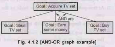
AO* Search and Problem Reduction Using AO*

When a problem can be divided in a set of sub problems, where each sub problem can be solved seperately and a combination of these will be a solution. AND-OR graphs or AND-OR trees are used for representing the solution.

AND-OR graphs

1) The decomposition of the problem or problem reduction generates AND arcs.

2) One AND arc may point to any number of successor nodes.

3) All these must be solved so that the man the arc will give rise to many arcs, indicating several possible solutions.Hence the graph is known as AND-OR instead of AND.

4) AO* is a best-first algorithm for solving problems represented as a cyclic AND/OR graphs problems.

5) An algorithm to find a solution in an AND-OR graph must handle AND area appropriately.

The comparative study of A* and AO*

1) Unlike A* algorithm which used two lists OPEN and CLOSED, the AO* algorithm uses a single structure G.

2) G represents the part of the search graph generated so far.

3) Each node in G points down to its immediate successors and upto its immediate predecessors, and also has with it the value of 'h' cost of a path from itself to a set of solution nodes.

4) The cost of getting from the start nodes to the current node 'g' is not stored as in the A* algorithm. This is because it is not possible to compute a single such value since there may be many paths to the same state.

5) AO* algorithm serves as the estimate of goodness of a node.

6) A* algorithm cannot search AND-OR graphs efficiently.

7) AO* will always find minimum cost solution.

• The algorithm for performing a heuristic search of an AND-OR graph is given below.

AO* algorithm

1) Initialize the graph to start node.

2) Traverse the graph following the current path accumulating nodes that have not yet been expanded or solved.

3) Pick any of these nodes and expand it and if it has no successors call this value as, FUTILITY, otherwise calculate only f' for each of the successors.

4) If 'f' is 0 then mark the node as SOLVED.

5) Change the value of 'f' for the newly created node to reflect its successors by back el to propagation.

6) Wherever possible use the most promising routes and if a node is marked as SOLVED then mark the parent node as SOLVED.

7) If starting node is SOLVED or value greater than FUTILITY, stop, else repeat from 2.

How to Search Better?

We have seen many searching strategies till now, but as we can see no one is really the perfect. How can we make our AI agent to search better?

We can make use of a concept called as metalevel state space. Each state in a metalevel state space captures the internal (computational) state of a program that is searching in an object-level state space such as in Indian Traveller Problem.

Consider A* algorithm

1) In A* algorithm it maintains internal state which consists of the current search tree.

2) Each action in the metalevel state space is computation step that alters the internal state.

For example - Each computation step in A* expands a leaf node and adds its successors to the tree.

3) As the level increases the sequence of larger and larger search trees is generated.

In harder problem there can be mis-steps taken by algorithm. That is algorithm can explore unpromising unuseful subtrees. Metalearning algorithm overcomes these problems.

The main goal of metalearning is to minimize the total cost of problem solving.

Heuristic Functions and their Nature

1. Accuracy of Heuristic Function

• More accurate the heuristic function more is the performance.

• The quality of heuristic function can be measured by the effective branching factor b*.

• Consider A* that generates N nodes and 'd' is depth of a solution, then b* is the qulay branching factor that a uniform tree of depth 'd' would have so as to contain 'n+1' nodes.

Thus,

  N+1 = 1 + b* + (b*)² + ... + (b*)^d

If A* finds a solution at depth 5 using 52 nodes, then the effective branching factor is 1.92.

A well designed heuristic function will have a value of b* close to 1, allowing fairly large problems to be solved.

2. Designing Heuristic Functions for Various Problems

Example 4.1.1 8-puzzle problem.

Solution: The objective of the puzzle is to slide the tiles horizontally or vertically into the empty space until the configuration matches the goal configuration.

1) The average solution cost for a randomly generated 8-puzzle instance is about 22 steps.

2) The branching factor is about 3 (when the empty tile is in the middle, there are no four possible moves, when it is in a corner there are two, and when it is along an edge there are three.

3) An exhaustive search to depth 22 would look at about 3²² ≈3.1×10¹⁰ states.

4) If we keep track of repeated states, we could cut this down by a factor of about 1,70,000, because there are only 9!/2 = 1,81,440 distinct states that are reachable.

5) If we use A*, we need a heuristic function that never overestimates the number of steps to the goal.

6) We can use following heuristic function,

-h₁ = The number of misplaced tiles. All of the eight tiles are out of position, so the start state would have h1 =8.h1, is an admissible heuristic, because it is clear that any tile that is out of place must be moved at least once.

- հ₂ = The sum of the distances of the tiles from their goal positions. Because tiles cannot move along diagonals, the distance we will count is the sum of the horizontal and vertical distances.

Example 4.1.2 Blocks world problem.

Solution:

Heuristic for Blocks World

A function that estimates the cost of getting from one place to another (from the current state to the goal state.)

Used in a decision process to try to make the best choice of a list of possibilities (to choose the move more likely to lead to the goal state.)

Best move is the one with the least cost.

The "intelligence" of a search process, helps in finding a more optimal solution.

h1(s)= Number of places with incorrect block immediately on top of it.

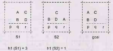
A more informed heuristic

Looks at each bottom position, but takes higher positions into account. Can be broken into 4 different cases for each bottom position.

1. Current state has a blank and goal state has a block.

Two blocks must be moved onto q. So increment the heuristic value by the number of blocks needed to be moved into a place.

2. Current state has a block and goal state has a blank.

One block must be removed from P. So increment the heuristic value by the number of blocks needed to be moved out of a place.

3. Both states have a block, but they are not the same.

On place q, the blocks don't match. The incorrect block must be moved out and the correct blocks must be moved in. Increment the heuristic value  by the number of these blocks.

4. Both states have a block, and they are the same.

B is in the correct position. However, the position above it is incorrect. Increment the heuristic value by the number of incorrect positions above the correct block.

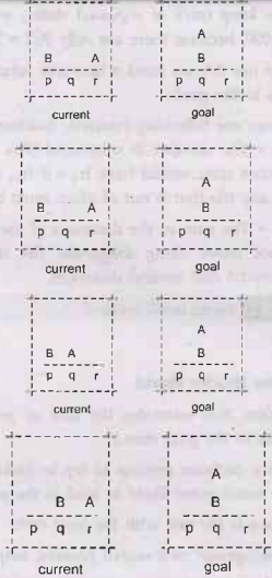
Example

Know the second state leads to the optimal solution, but not guaranteed to be chosen first. Can the heuristic be modified to decrease its value? Yes, since the block on p can be moved out and put on q in the same move. Need to compensate for this overcounting of moves.

For a given (nonempty) place, find the top-most block. Look for its position in the goal state. If it goes on the bottom row and the place is currently empty, the block can be moved there, so decrement heuristic by one.

Now the second state's heuristic will be 3, and it's guaranteed to be chosen before the other one. A little like a one move look ahead.

If the top-most block doesn't go on bottom row, but all blocks below it in the goal state are currently in their correct place, then the block can be moved there, so decrement heuristic by one.

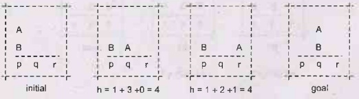
Example

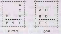
p: case 4: +1

q: case 1: +2

r: case 2: +3

A can beput on B: -1

so h=5

optimal number of moves is 4

Example 4.1.3 Travelling salesman problem.

Solution: Heuristic function, h(n) is defined as,

h(n) = estimate cost of the cheapest path from node 'n' to a goal state.

Heuristic function for Travelling salesman problem:

• Travelling salesman problem (TSP) is a routing problem in which each city must be visited exactly once. The aim is to find the shortest tour.

• The goal test is, all the locations are visited and agent at the initial location.

• The path cost is distance between locations.

• As a heuristic function for TSP, we can consider the sum of the distances travelled T so for. The distance value directly affects the cost therefore, it should be taken into calculation for heuristic function.

Heuristic function for 8 puzzle problem.

• The objective of the 8 puzzle is to slide the tiles horizontally or vertically into the empty space until the configuration matches the goal configuration.

• We can use following heuristic function,

• h₁ = The number of misplaced tiles. All of the eight tiles are out of position, so the start state would have h1 = 8.h1, is an admissible heuristic, because it is logo clear that any tile that is out of place must be moved at least once.

• h₂ = The sum of the distances of the tiles from their goal positions. Because tiles cannot move along diagonals, the distance we will count is the sum of the horizontal and vertical distances.

Example 4.1.4 Tic Tac Toe problem.

Solution: Heuristic for Tic Tac Toe problem

This problem can be solved all the way through the minimax algorithm but if a simple heuristic/evaluation function can help save that computation. This is a static evaluation function which assigns a utility value to each board position by assigning weights to each of the 8 possible ways to win in a game of tic-tac-toe and then summing up those weights.

One can evaluate values for all of 9 fields, and then program would choose the field with highest value.

For example,

Every Field has several WinPaths on the grid. Middle one has 4 (horizontal, vertical and two diagonals), corners have 3 each (horizontal, diagonal and one vertical), sides have only 2 each (horizontal and vertical). Value of each Field equals sum of its WinPaths values. And WinPath value depends on its contents:

• Empty [| |] - 1 point

• One symbol: [X | | ] - 10 points // can be any symbol in any place

• Two different symbols: [X | O | ] -.0 points // they can be arranged in way

• Two identical opponents symbols: [X | X | ] - 100 points // arranged any of three way

• Two identical "my" symbols: [O | O | ] - 1000 points // arranged in any of three ways

• This way for example beginning situation has values as below:

3. Domination of Heuristic Function

• If we could design multiple heuristic function for same problem then we can find that which one is better.

• Consider two heuristic functions h1 and h2. From their definitions for some node n, if h2 (n) ≥ h1(n) then we say that h2 dominates h1.

• Domination directly points to accuracy, A* using h2 will never expand more nodes than A* using h1 (except for some node having f(n) = c*)

4. Admissible Heuristic Functions

1) A problem with fewer restrictions on actions is called a relaxed problem.

2) The cost of an admissible solution to a relaxed problem is an admissible heuristic not for the original problem. The heuristic function is admissible because the optimal solution in the original problem is, also a solution in the relaxed problem, and therefore must be at least as expensive as the optimal solution in the relaxed problem.

3) As the derived heuristic is an exact cost for the relaxed problem, therefore it is consistant.

4) If problem definitions are written in formal languages then it is possible to construct relaxed problem automatically.

5) Admissible heuristic function can also be derived from the solution cost of a subproblem of the given problem. The cost of optimal solution of this subproblem would be the lower bound on the cost of the complete problem.

6) We can store the exact solution costs for every possible subproblem instance in a database. Such a database is called as pattern database.

The pattern database is constructed by searching backwards from the goal state and recording the cost of each new pattern encountered.

We can compute an admissible heuristic function 'h' for each complete state encountered during a search simply by looking up the corresponding subproblem configuration in the database.

7) The cost of the entire problem is always greater than sum of cost of two subproblems. Hence it is always better to derive disjoint solution and then sum up all solutions to minimize the cost.

Learning Heuristic from Experience

1) A heuristic function h(n) is supposed to estimate the cost of a solution begining from the state at node n. Therefore it is really difficult to design h(n).

2) One solution is to devise relaxed problems for which an optimal solution can be found.

3) Another solution is to make agent program that can learn from experience.

- "Learn from experience" means solving similar problem again and again (i.e. practicing).

- Each optimal solution will provide example from which 'h(n) design' can be learned.

- One can get experience of which h(n) was better.

- Each example consists of a state from the solution path and the actual cost of the solution from that point.

- From such solved examples an inductive learning algorithm can be used to construct the function h(n) that can predict solution costs for another states that have arised during search. [A lucky agent program will get the prediction early.]

For developing inductive algorithms we can make use of techniques like neural nets, decision trees, etc.

If inductive learning methods have knowledge about features of a state that are relevant to evaluation of algorithms then inductive learning methods give of oldies best output.