Search Strategies

Search Strategies

AU Dec.-09, 13, 14, 16, May-10, 12, 13, 14, 15

At every stage in state space generating algorithms we need to apply searching procedure so as to reach to goal state. Search is a systematic examination at states to find path from the root state (initial state) to the goal state. The output of this procedure is the solution (goal) state.

Two Basic Search Strategies

1) Uninformed search (Blind search): They have no additional information about states other than provided in the problem definition.

They can only generate successors and distinguish between goal state and non-goal state.

2) Informed search (Heuristic search): This can decide whether one non-goal state is more promising than another non-goal state.

Key Point All the search strategies are distinguished by the order in which the nodes are expanded.

Uninformed Search Strategies

1. B.F.S.

2. D.F.S.

3. Depth limited search

4. Iterative deepening DFS

5. Bidirectional search

6. Uniform cost search

In the following section we will discuss each uninformed searching in detail. For each searching technique we will see its basic methodology, its algorithmic implementation and its performance evaluation. Performance evaluation will be done on the basis of 4 criterias we have seen previously namely,

1) Completeness

2) Optimality

3) Time complexity

4) Space complexity.

Generally it does happen that space and time complexity depends on some factors hence we will discuss them combinely.

1. Breadth-First Search

The procedure: In BFS root node is expanded first, then all the successor of root node are expanded and then their successor and so on. That is the nodes are expanded level wise starting at root level.

The implementation: BFS can be implemented using first, in first out queue data structure where fringe will be stored and processed. As soon as node is visited it is added to queue. All newly generated nodes are added to the end of the queue, which means that shallow nodes are expanded before deeper nodes.

The performance evaluation

1) Completeness: BFS is complete because if the shallowest goal node is at some finite depth d, BFS will eventually find it and will generate solution. (assuming that branching factor b is finite).

2) Optimality: The shallowest goal node is not necessarily optimal. BFS will yield optimal solution only when all actions have the same cost, let it be at any depth.

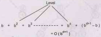
3) Time and space complexity: As the level of search tree grows more time is incurred. In general if search tree is at level d then O (b^d+1) time is required, where b is the number of nodes generated from each node, starting at root node i.e. root generates b nodes and each b node generates b more and so on shown below.

Every node generated should remain in memory till its exploration. If branching factor 'b' is more then more memory will be required.

For example-

If branching factor b = 10 at some level d = 6. If we assume 10,000 nodes will be generated per second and per node 1000 bytes are required for storage.

Then total generated nodes = 10⁷ which will take 19 minutes but it will take 10 Gigabytes for storing them.

We can conclude that for BFS space complexity is major issue concerned than time complexity. Time complexity is critical issue when depth of tree increases.

Key Point We can use uninformed methods for exponential-complexity search only when problems have smallest instances.

Algorithm BFS (G, n)

//Breadth first search of G

{

for i := 1 to n do // Mark all vertices unvisited

visited [i] = 0;

for i = 1 to n do

if (visited [i] = 0) then BFS (i);

}

BFS

• Time complexity - O(b ^d+1)

• Space complexity - O(b ^d+1)

BFS

D and J are goal state.

[D is found through the path] → (A-B-D) (shallowest goal)

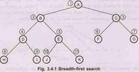
Note The numeric value beside each node indicates the order in which nodes are visited (reached).

2. Uniform Cost Search

The procedure: Uniform cost search expands the node. 'n' with the lowest path cost. Uniform cost search does not care about the number of steps a path has, instead it considers their total cost. Therefore, their is a chance of getting stuck in an infinite loop if it ever expands a node that has a zero-cost action leading back to the same state.

The implementation: We can use queue data structure for storing fringe as in BFS. The major difference will be while adding the node to queue, we will give priority to the node with lowest pathcost. (So the data structure will be a priority queue).

The performance evaluation

1) Completeness: Uniform cost search guarantees completeness provided the cost of every step is greater than or equal to some small positive constant "c".

2) Optimality: If cost of every step is greater than or equal to some small positive constant then uniform cost search will yeild optimal solution, by reaching the goal state which has lowest path cost.

3) Time and space complexity: Uniform-cost search does not care about the number of steps a path has, but only about their total cost. Therefore, it will get stuck in an infinite loop if it ever expands a node that has a zero-cost action leading back to the same state.

Uniform-cost search is guided by path costs rather than depths, so its complexity cannot easily be characterized in terms of b and d. Instead, let C* be the cost of the optimal solution, and assume that every action costs at least E. Then the algorithm's worst-case time and space complexity is O (b[C*/ϵ]), which can be much greater than bd.

Uniform cost search

• Time complexity - O (b^C/ϵ)

• Space complexity - O (b^C/ϵ)

where - C is the cost of optimal solution.

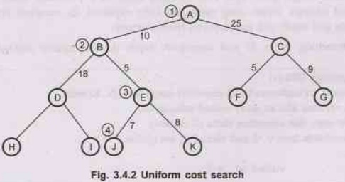
Assuming J and D are both goal state.

A – B – E – J

Note The costs are associated with each edge.

Note The numeric value beside each node indicates the order in which nodes arevisited (reached).

3. Depth-First Search

The procedure: Depth-first search always expands the deepest node in the current unexplored node set (fringe) of the search tree. The search goes in to depth until there is no more successor node. As these nodes are expanded, they are dropped from the fringe, so then the search "backs up" to the next shallowest node (previous level node) that still has unexplored successors.

The implementation: DFS can be implemented with stack (LIFO) data structure which will explore the latest added node first, suspending exploration of all previous nodes on the path. This can be done using recursive procedure that calls itself on each of the children in turn.

The performance evaluation    

1) Completeness: As DFS explores all the nodes hence it guareentees the solution.

2) Optimality: As DFS reach to deepest node first, it may ignore some shallow node which can be goal state. Therefore optimality is expected only when all states have same path cost.

3) Time and space complexity: DFS requires some moderate amount of memory as it needs to store single path from root to some node to a particular level, along with unexpanded siblings. When same node gets fully explored, its complete branch (its all descendants and itself) will get removed from memory.

With branching factor 'b' and maximum depth d, dfs requires storage of - bd+1 nodes.

Algorithm DFS (v)

//Given an undirected (OR directed) graph G = (V, E) with

//n vertices and an array visited initially set

// to zero, this algorithm visits all vertices

//reachable from v. G and visited [ ] are global.

{

visited [v] : = 1;

for each vertex w adjacent from v do

{

if (visited [w] = 0 then DFS (w);

}

}

• Time complexity – O (b^d).

• Space complexity – O (b^d +1).

4. DFS [Depth First Search]

Goal state path - (A - B - D)

where D is a goal state.

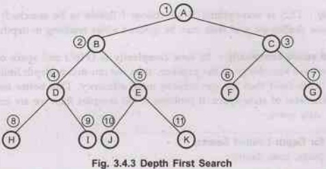
Note The numeric value beside each node indicates the order in which nodes are visited (reached).

A special case DFS → back tracking search: In this only one successor is generated at a time rather than all the successors and each partially expanded node remembers which successor to generate next.

This search technique uses less memory than DFS as only 'd' nodes (maximum depth) are required to store.

Drawback of DFS: DFS can make a wrong choice and get stuck going down a very long (even infinite) path when a different choice would lead to a solution near the root of the search tree.

5. Depth-Limited Search (DLS)

The procedure: If we can limit the depth of search tree to a certain level then searching will be more efficient. This removes the problem of unbounded trees. Such a kind of depth first search where in the depth is limited at a certain level is called as depth limited search. It solves infinite path problem.

The implementation: Same as DFS but limited to depth level 1. DLS will terminate with two kinds of failure. The standard failure value indicates no solution and the cut-off value indicates no solution within the depth limit.

The performance evaluation                                                                         

1) Completeness: DLS suffers from completeness because if we choose 1 (levels to be searched) < d (actual levels), when shallowest goal is beyond the depth limit 1. It generally happens when 'd' is unknown.

2) Optimality: DLS is non-optimal if we choose I (levels to be searched) > d (actual levels) because shallowest goal state may be ignored while reaching to depth level l.

3) Time and space complexity: Its time complexity is O (b') and space complexity is O (bl). If we have knowledge of the problem, then we can decide depth limits. If we can find better depth limit then we can achieve more efficiency. This better depth limit is termed as diameter of state space. If problem is too complex then we are unable to find diameter of state space.

Algorithm for Depth Limited Search

DLS (node, goal, depth)

{

if(depth >=0)

{

if(node ==goal)

return node

for each child expand(node)

DLS (child, goal, depth-1)

}

}

General steps for DLS

1. Determine the node where the search should start and assign the maximum search depth.

2. Check if the current node is the goal state.

- IF not: Do nothing

- IF yes: Return

3. Check if the current node is within the maximum search depth.

- IF not: Do nothing

- IF yes: a) Expand the vertex and save all of its successors in stack.

      b) Call DLS recursively for all nodes of the stack and go back to step 2.

DLS [Depth-Limited Search]

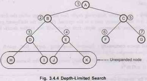
If depth limit = 2 then nodes on level 2 are not expanded.

D found (A-B-D)

(D, E, F, G are generated but not expanded).

J though better goal than D could not reached because of algorithm technique. 

Note The numeric value beside each node indicates the order in which nodes are visited (reached).

6. Iterative-Deepening Depth-First Search (IDDFS)

The procedure: In iterative deepening depth-first search, dfs is applied along with the best depth limit. In each step gradually it increases the depth limit until the goal is found. It increases depth limit from level 0, then level 1, then level 2 till the shallowest goal is found at certain depth 'd'.

The implementation: Iterative deepening depth first search can be implemented similar to BFS (where queue is used for storing fringe) because it explores a complete layer of new nodes at each iteration before going on to the next layer.

If we want to avoid memory requirements which are incurred in BFS then IDDFS can be implemented like uniform-cost search.

The key point is to use increasing path-cost limits instead of increasing depth limits, is if we have such a implementations it is termed as iterative lengthing search.

The performance evaluation

1) Completeness: It guarantees completeness as the search does not stop until goal node is found.

2) Optimality: As iterative deepening depth first search stops when the first goal node is reached, it is not necessary that it is the optimal. (That is, the shallowest goal reached is the final. Iterative deepening depth first search will not further search for optimal solution).

3) Time and space complexity: Iterative deepening depth first search has very moderate space complex which is O (b^d).

Its time complexity depends on branching factor (b) and the bottom most level that is depth (d). It is O (b^d).

Algorithm for Iterative-Deepening Depth First Search

//In IDDFS algorithm we are using DLS algorithm from earlier section IDDFS (root, goal)

{

depth = 0

while (no solution)

{

solution = DLS(root, goal, depth)

depth depth+1

}

return solution

}

• Example - IDDFS (Iterative Deepening Depth-First Search]

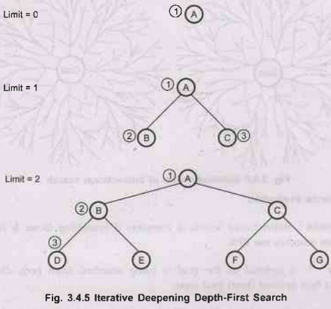
Note The numeric value beside each node indicates the order in which nodes are visited (reached).

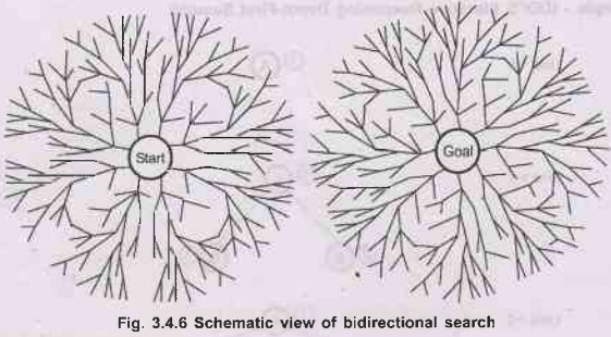
7. Bidirectional Search

The procedure: As the name suggests bi-directional that is two directional searches are made in this searching technique. One is the forward search which starts from initial state and the other is the backward search which starts from goal state. The two searches stop when both the searches meet in the middle. [As shown in below diagram].

The implementation: Bidirectional search is implemented by having one or both of the searches check, each node before it is expanded, is examined to see if it is in the fringe of the other search tree. If so solution is found. Fringe can be maintained in queue data structure, like BFS.

The performance evaluation

1) Completeness: Bidirectional search is complete if branching factor b is finite and both directions searches use BFS.

2) Optimality: It is optimal as the goal is being searched from both directions. So guaranteed to find optimal (best) goal state.

3) Time and space complexity: Bidirectional search has time complexity as O (b ^d/2), where 'b' is branching factor. It is the important noticable point in case of backward a search because, we need to get predecessors of the node. The easiest case is when all the actions in the state space are reversible.

When one goal state is there, the backward search is very much like the forward search (like in 8 puzzle problem). If there are several explicitly listed goal states (like in part picking robot) then it needs to construct a new dummy goal state whose immediate predecessors are all then actual goal states. The worst case in bidirectional search is when the goal test gives only implicit description of some possibly large set of goal states.

For example, in the game of chess 'checkmate' is the goal state which will have many possible description.

The memory requirement for bidirectional search is also moderate which is O (b^d/2) where b = Branching factor, d = Depth, where at least one of the search tree is maintained in memory.

Bidirectional search

Space complexity - O (b^d/2)

Time complexity - O (b^d/2)