Scheduling Algorithms

Scheduling Algorithms

AU: Dec.-17, May-17, 18, 19, 22

• CPU scheduling algorithms are as follows:

1. First In First Out (FIFO) scheduling        

2. Shortest job first scheduling

3. Priority scheduling

4. Round robin scheduling

First Come First Serve Scheduling

• This method of scheduling means that the first process to request the processor gets it until it finished execution. With this algorithm, processes are assigned the CPU in the order they request it.

• Normally there is a single queue of ready processes. When the first process enters the system from the outside, it is started immediately and allowed to run as long as it wants it. At the same time, other process enters into the system; they are put onto the end of the queue.

•  New process enters the tail of the queue and the schedule selects the the head of the queue.

• When new process enters into the system, its process control block is linked to the end of the ready queue and it is removed from the front of the queue.

• When a process waits or blocks, it is removed from the queue and it queues up Anton again in FCFS queue when it gets ready.

• FCFS is non-preemptive CPU scheduling algorithm. It is also called First In First Out method (FIFO).

• FCFS is simple to implement because it uses a FIFO queue. This algorithm is fine for most of the batch operating systems.

• FCFS is not useful in scheduling interactive processes because it cannot guarantee short response time. This algorithm performs much better for long processes than and it short ones.

• Turnaround time is unpredictable with the FCFS algorithm. Average waiting time of the FCFS is often quite long.

• Real life analogy is buying tickets.

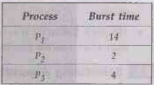
Example 2.6.1 Consider the following set of process that arrives at time 0, with the length of the CPU burst given in milliseconds

Calculate the average waiting time.

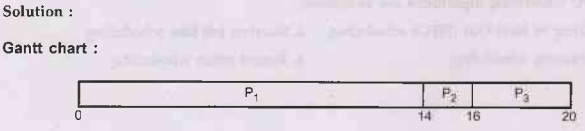
Such a diagram is called "Gantt charts", showing when each CPU burst uses the CPU. Here, each CPU burst comes from a different thread.

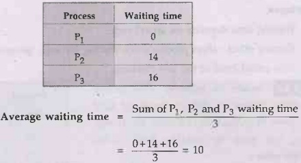
Waiting Time :

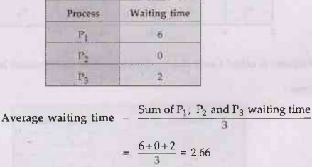
• If the processes change their order of arrive i.e. P2, P3, P1, then the results will be different than first one and it is shown below:

Gantt chart:

Waiting Time :

Convey effect

• To reduce I/O device utilization, all I/O bound processes will be waiting excessively long for processor bound ones. This is called as convey effect.

• If one process monopolizes the system, the extent of its overall effect on system performance depends on the scheduling policy and whether the process is processor bound or I/O bound.

Advantages

1. Simple to implement

2. Fair

Disadvantages

1. Waiting time depends on arrival order

2. Convoy effect: short process stuck waiting for long process

3. Also called head of the line blocking

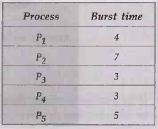
Example 2.6.2 Consider the following set of process that arrive at time 0, with the length of CPU burst given in milliseconds. Calculate the average waiting time when the processes arrive in the following order:

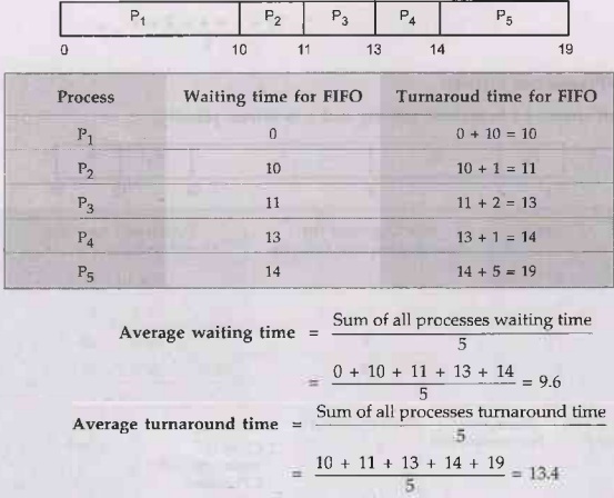
a. P1, P2, P3 P4 P5

Provide the Gantt chart for the same.

Solution :

Gantt chart :

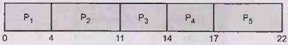
Such diagram is called Gantt charts, showing when each process burst uses the CPU.

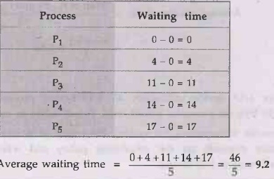
Waiting time:

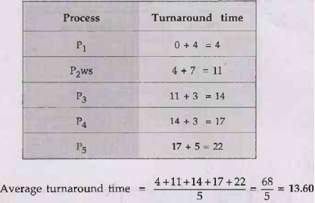
Turnaround time: Turnaround time = Waiting time + Burst time

Shortest Job First Scheduling

• Shortest job first scheduling algorithm is also known as Shortest Job Next (SJN) scheduling algorithm. It handles the process based on length of their CPU cycle time. It reduces average waiting time over FIFO algorithm.

• SJF is a non-preemptive CPU scheduling algorithm.

• It does not work in interactive system because users do not estimate in advance the CPU time required to run their processes.

• SJF scheduling algorithm is used frequently in long term scheduling.

• When a process request a CPU, it must inform the system for how long it wants to use the CPU.

• When CPU become available, the system allocates into processes with the least expected execution time.

• To break ties, it follows the FCFS algorithm.

• Preemptive version of SJF is called as Shortest Remaining Time Next (SRTN)

• Preemptive SJF algorithm will preempt the currently exceuting process, whereas a non preemptive SJF algorithm will allow the currently running process to finish its CPU burst.

• SIF selects processes for service in a manner ensuring the next one will complete and leave the system as soon as possible.

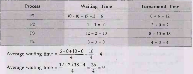
Example 2.6.3 Calculate the average waiting time and average turnaround time. Provide the Gantt chart for the same.

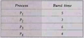
Solution :

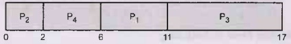
Gantt chart:

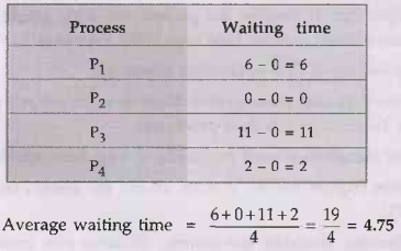
Waiting time :

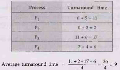
Turnaround time: Turnaround time = Waiting time + Burst time

• The SJF scheduling algorithm is optimal only when all of the processes are available at the same time and the CPU estimates are available.

• SJF scheduling algorithm may be preemptive or non-preemptive.

Priority Scheduling

• Priority CPU scheduling algorithm is preemptive and non-preemptive algorithm. It is one of the most common scheduling algorithm in batch system. Priority can be assigned by a system admin using characteristics of the process.

• In this scheduling algorithm, CPU select higher priority process first. If the priority of two process is same then FCFS scheduling algorithm is applied for solving the problem.

• The priority of a process determines how quickly its request for a CPU will be granted if other processes make competing requests.

• Each process is assigned a priority number for the purpose of CPU scheduling.

• The priority number is normally a non negative integer number.

• Non preemptive priority scheduling algorithm will simply put the new process at the head of the ready queue.

• Preemptive priority scheduling algorithm will preempt the CPU if the priority of the newly arrived process is higher than the priority of the currently running process.

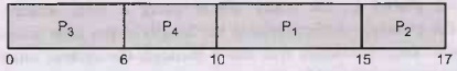
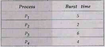
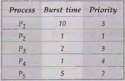
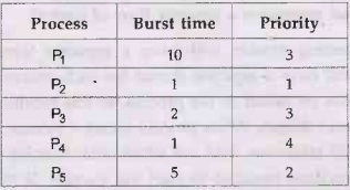
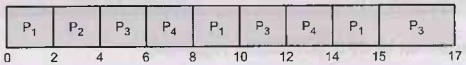
Example 2.6.4 Consider the following set of process that arrive at time 0, with the length of CPU burst given in milliseconds. Calculate the average waiting time and average turnaround time. Provide the Gantt chart for the same. (Time slice = 2)

Solution: For non-preemptive priority scheduling

Gantt chart :

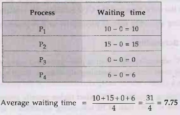
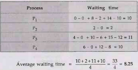
Waiting time:

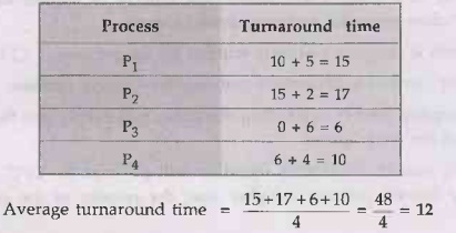
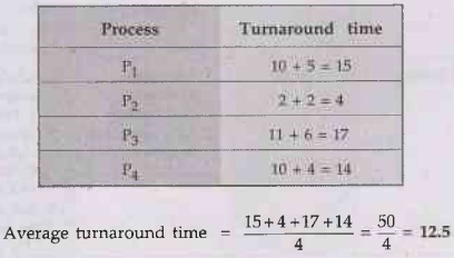
Turnaround time: Turnaround time = Waiting time + Burst time

Problem with Priority Scheduling

• Waiting time is more for lower priority process even if there required CPU burst time is less. Priority scheduling algorithm faces the starvation problem. Starvation problem can be solved by using aging techniques.

• In aging, the priority of the process will increase which is waiting for long time in the ready queue.

Round Robin Scheduling

• Round robin is a preemptive scheduling algorithm. It is used in interactive system. Here process are given a limited amount of time of processor time called a time slice or time quantum. If a process does not complete before its quantum expires, the system preempts it and gives the processor to the next waiting process. The system then places the preempted process at the back of the ready queue.  

• Processes are placed in the ready queue using a FIFO scheme. With the RR algorithm, the principle design issue is the length of the time quantum to be used. For short time slice, processes will move through the system relatively quickly. It increases the processing overheads.

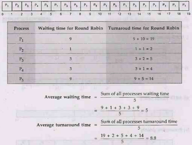
Example 2.6.5 Consider the following set of process that arrive at time 0, with the length of CPU burst given in milliseconds. Calculate the average waiting time and average turnaround time. Provide the Gantt chart for the same. (Time slice = 2)

Solution:

Gantt chart:

Waiting time :

Turnaround time: Turnaround time = Waiting time + Burst time

Comparison between FCFS and RR

Comparison of CPU Scheduling Algorithm

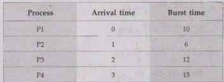
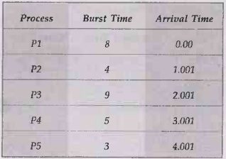
Example 2.6.6 Consider the following process, with the CPU burst time given in milliseconds.

Processes are arrived in P1, P2, P3, P4 P5 order at time 0.

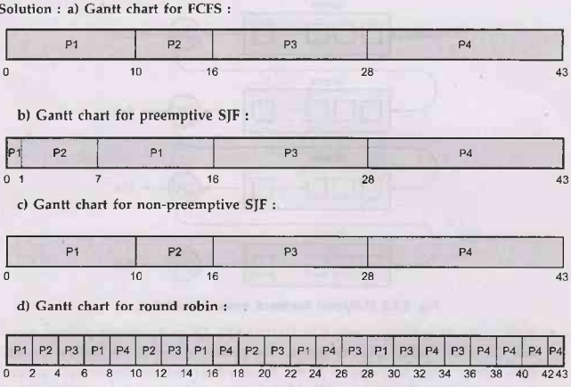
(i) Draw four Gantt charts to show execution using FIFO, SJF, non-preemptive priority and Round Robin (Quantum = 1) scheduling.

(ii) Also calculate waiting time and turnaround time for each scheduling algorithm.  AU May-18, Marks 15

Solution :

1) FIFO: Gantt chart:

2) SJF: Gantt chart:

3) Non-Preemptive Priority

Gantt chart: (1 is highest priority and 4 is lowest priority)

4) Round Robin (Quantum = 1)

Gantt chart:

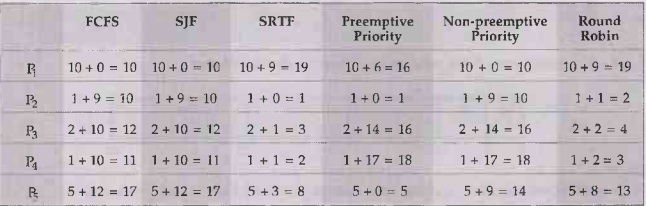
Example 2.6.7 Consider the following set of processes with the length of CPU - burst time given in milliseconds.

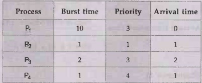
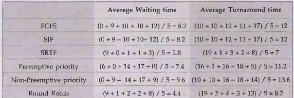
Draw the Gantt chart for execution of these processes using FCFS, SJF, SRTS, pre-emptive and non-pre-emptive priority, round robin with time slice of 2 ms. Find the average waiting and turnaround time using each of the methods.  AU :May-19,Marks 10

Waiting time:

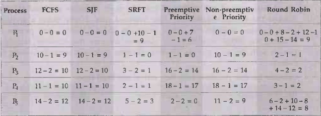
Turnaround time

Average waiting time and turnaround time

Shortest Remaining Time Next

• Preemptive SJF is called shortest remaining time first. In this algorithm, the scheduler selects the process with the smallest estimated run time to completion. 

• This scheduler gives minimum wait times in theory but in certain situation due to preemption overhead, shortest process first might performance better.

• An advantageous of this method is that, the short processes are handled very quickly. The system requires very little overhead since it only makes a decision when a process completes or a new process is added. When a new process is admitted the SRTN algorithm only needs to compare the currently executing process with the new process, ignoring all other processes currently waiting to execute.

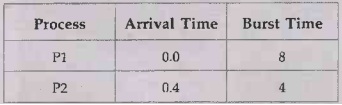
• Consider the four processes with their arrival and burst time.

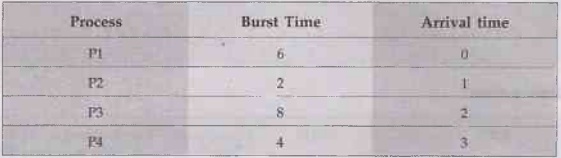
• The execution of the process is shown by the Gantt chart:

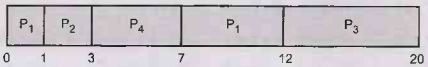
• Now we calculate waiting time and turnaround time for all processes.

Advantages:

1. Very short processes get very good service.

2. The penalty ratios are small; this algorithm works extremely well in most cases 

3. This algorithm pravably gives the highest throughput of all scheduling algorithms if the estimates are exactly correct.

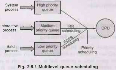
Multilevel Queue Scheduling

• Multilevel queue is not separate scheduling algorithm but it works in conjunction with several CPU scheduling algorithms. The processes can be grouped according to common characteristics.

• One type of multilevel queue is based on the priority based system with different queues for each priority level.

• System consists of two types of processes or jobs: Interactive and batch. Interactive jobs are shorter and batch jobs are longer. Fig. 2.6.1 shows multilevel queue scheduling.

• To keep minimum response time for user, interactive jobs are scheduled before the batch jobs. So ready queue is partitioned into two separate queue: interactive (foreground) and batch (background). Each queue uses their own scheduling algorithm.

• Once the jobs assigns to the queue, it will remain in that queue. Jobs never change the queue. Here we assume that FCFS is applied to one queue and round robin method is applied to another queue.

•The batch jobs are put in one queue called the background queue while the interactive jobs are put in a foreground queue. Batch jobs are scheduled by first come first serve method and interactive jobs by round robin method.

• The scheduler now has to decide which queue to run. The methods are as follows:

  1. Higher priority queues can be processed until they are empty before the lower priority queues are executed.  

  2. Each queue can be given a certain amount of the CPU. Maybe, the interactive queue could be assigned 75 % of the CPU, with the batch queue being given  25 %.

• It should also be noted that there can be many other queues. Many systems will have a system queue. This queue will contain processes that are important to keep the system running. For this reason these processes normally have the highest priority.

• It should be also need to specify which queue a process will be put to when it arrives to the system and/or when it starts a new CPU burst.

Advantages:

1. It can be preemptive or non-preemptive.

2. Short CPU bound processes are executed first.

3. Simple to implement.

Disadvantage :

1. Queues require monitoring, which is a costly activity.

Multilevel Feedback Queue Scheduling

• Multilevel Feedback Queue (MLFQ) allows moving the processes between the queues. MLFQ has a number of distinct queues; each assigned a different priority level. At any given time, a process that is ready to run is on a single queue. MLFQ uses priorities to decide which process should run at a given time. A process with higher priority is selected for execution.

• Consider processes with different CPU burst characteristics. If a process uses too much of the CPU it will be moved to a lower priority queue. This will leave I/O bound and interactive processes in the higher priority queue.

• Fig. 2.6.2 shows multilevel feedback queue scheduling. (See Fig. 2.6.2 on next page.)

• MLFQ also uses concept of aging to prevent starvation. The processes with lower priority will move towards the higher priority queue in aging concept. The key to MLFQ scheduling lies in how the scheduler sets priorities. Rather than giving a fixed priority to each process, MLFQ varies the priority of a process based on its observed behavior.

• Assume we have three queues (Q0, Q1 and Q2). Q0 is the lowest priority queue and Q2 is the highest priority queue. The process enters at the highest priority ESA (Q2). After a single time-slice of 10 ms, the scheduler reduces the process's priority by one, and thus the job is on Q1. After running at Q1 for a time slice, the job is finally lowered to the lowest priority in the system (Q0), where it remains.

• Following parameters are defined by scheduler for implementing MLFQ:

1. Number of queue required.

2. Scheduling algorithm for each queue.

3. Method is required for finding to increase and/or decrease priority of processes.

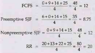
Example 2.6.8 Explain the FCFS, preemptive and non preemptive versions of shortest-job-first and roudn robin (time slice = 2) schedulign algorithms with Gantt chart for the four processes given. Compare their average turn around and waiting time.

Waiting time

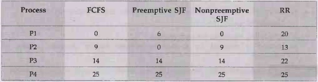
AverageWaiting time

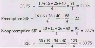
Turnaround time

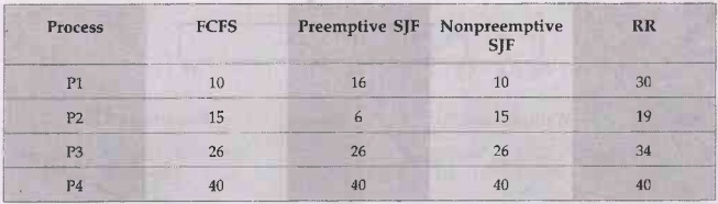
Average Turnaround time

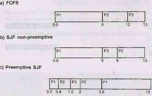
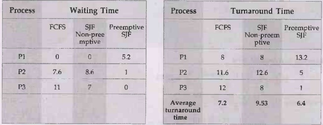
Example 2.6.9 What is the average turnaround time for the following process using a) FCFS b) SJF non-prrmptive c) Preemptive SJF.

AU Dec.-17, Marks 9

 

Solution: Gantt chart:

University Questions

1.Consider the following set of processes, with the length of the CPU-burst time in given ms:

Draw four Gantt charts illustrating the execution of these processes using FCFS, SJF, priority and RR (quantum = 2) scheduling. Also calculate waiting time and turnaround time for each scheduling algorithms.  AU May-17, Marks 13

2. Explain the differences in the degree to which the following scheduling algorithms discriminate in favor of short process. :

i) RR ii) Multilevel feedback queues.  AU May-18, Marks 13

3. Consider the following set of processes, with the length of the CPU burst given in milliseconds :

The process are assumed to have arrived in the order P1, P2, P3, P4, P all at time 0.

i) Draw Gantt chart that illustrate the execution of these processes using the scheduling algorithms FCFS (smaller priority number implies higher priority) and RR (quantum = 1).[10]

ii) What is the waiting time of each process for each of the scheduling algorithms. [5]  AU: May-18,22, Marks 15

4. Explain - multi level queue and multi level feedback queue scheduling with suitable examples.  AU :May-19,Marks 05