Artificial Intelligence and Machine Learning: Unit III: Supervised Learning
Regression
Supervised Learning - Artificial Intelligence and Machine Learning
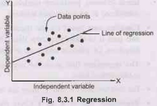
Regression finds correlations between dependent and independent variables. If the desired output consists of one or more continuous variable, then the task is called as regression.
Regression
•
Regression finds correlations between dependent and
independent variables. If the desired output consists of one or more continuous
variable, then the task is called as regression.
•
Therefore, regression algorithms help predict
continuous variables such as house prices, market trends, weather patterns, oil
and gas prices etc.
•
Fig. 8.3.1 shows regression.
•
When the targets in a dataset are real numbers, the
machine learning task is known as regression and each sample in the dataset has
a real-valued output or target.
•
Regression analysis is a set of statistical methods
used for the estimation of relationships between a dependent variable and one
or more independent variables. It can be utilized to assess the strength of the
relationship between variables and for modelling the future relationship
between them.
•
The two basic types of regression are linear
regression and multiple linear regression.
8.3.1
Linear Regression
Models
•
Linear regression is a statistical method that allows
us to summarize and study relationships between two continuous (quantitative)
variables.
•
The objective of a linear regression model is to find
a relationship between the input variables and a target variable.
1. One
variable, denoted x, is regarded as the predictor, explanatory or buy
independent variable.
2.
The other variable, denoted y, is regarded as the response, outcome or
dependent variable.
•
Regression models predict a continuous variable, such
as the sales made on a day predict temperature of a city. Let's imagine that we
fit a line with the training point that we have. If we want to add another data
point, but to fit it, we need to change existing model.
•
This will happen with each data point that we add to
the model; hence, linear regression isn't good for classification models.
•
Regression estimates are used to explain the
relationship between one dependent variable and one or more independent
variables. Classification predicts categorical labels (classes), prediction
models continuous - valued functions. Classification is considered to be
supervised learning.
•
Classifies data based on the training set and the
values in a classifying attribute and uses it in classifying new data.
Prediction means models continuous - valued functions, i.e. predicts unknown or
missing values.
•
The regression line gives the average relationship
between the two variables in mathematical form.
•
For two variables X and Y, there are always two lines
of regression.
•
Regression line of X on Y Gives the best estimate for
the value of X for any specific given values of Y:
X =
a + b Y
Where a=
X - intercept
b = Slope
of the line
X =
Dependent variable
Y =
Independent variable
•
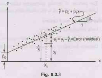
Regression line Y on X: Gives the best estimate for the
value of Y for any specific given values of X:
Y =
a + bx
Where
a = Y - intercept
b = Slope
of the line
Y =
Dependent variable
X =
Independent variable
•
By using the least squares method (a procedure that
minimizes the vertical deviations of plotted points surrounding a straight
line) we are able to construct a best fitting straight line to the scatter
diagram points and then formulate a regression equation in the form of :
y =
a + bx
y =
y +b(x-x)
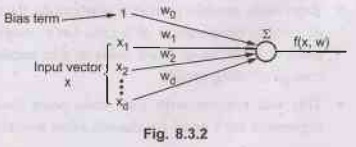
• Regression analysis is the art and science of fitting straight lines to patterns of data. In a linear regression model, the variable of interest ("dependent" variable) is predicted from k other variables ("independent" variables) using a linear equation. If Y denotes the dependent variable and X1,..., Xk, are the independent variables, then the assumption is that the value of Y at time t in the data sample is determined by the linear equation :
Y1 = β0 + β1 X1t + β2 X2t +...+ βk Xkt +εt
where
the betas are constants and the epsilons are independent and identically
distributed normal random variables with mean zero.
•
At each split point, the "error" between
the predicted value and the actual values is squared to get a "Sum of
Squared Errors (SSE)". The split point errors across the variables are
compared and the variable/point yielding the lowest SSE is chosen as the root
node/split point. This process is recursively continued.
•
Error function measures how much our predictions
deviate from the desired answers.
Mean-squared
error Jn = 1/n Σi = 1…n (yi
– f(xi))2
Advantages:
a.
Training a linear regression model is usually much faster than methods such as
neural networks.
b.
Linear regression models are simple and require minimum memory to implement.
c.
By examining the magnitude and sign of the regression coefficients you can
infer how predictor variables affect the target outcome.
Least squares
•
The method of least squares is about estimating
parameters by minimizing the squared discrepancies between observed data, on
the one hand, and their expected al values on the other.
•
Considering an arbitrary straight line, y = b0
+b1 x, is to be fitted through these data points. The question is
"Which line is the most representative"?
•
What are the values of b0 and b1
such that the resulting line "best" fits the data points? But, what
goodness-of-fit criterion to use to determine among all possible combinations
of nob b0 and b1?
•
The Least Squares (LS) criterion states that the sum
of the squares of errors is minimum. The least-squares solutions yields y(x)
whose elements sum to 1, but do not ensure the outputs to be in the range
[0,1].
•
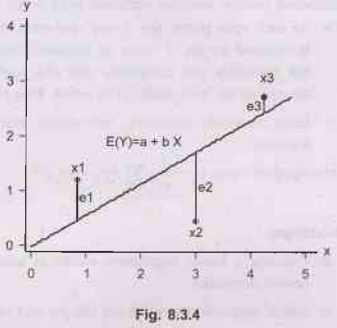
How to draw such a line based on data points
observed? Suppose a imaginary line of y = a + bx.
•
Imagine a vertical distance between the line and a
data point E = Y - E(Y).
•
This error is the deviation of the data point from
the imaginary line, regression line. Then what is the best values of a and b? A
and b that minimizes the sum of such errors.
•
Deviation does not have good properties for
computation. Then why do we use squares of deviation? Let us get a and b that
can minimize the sum of squared deviations rather than the sum of deviations.
This method is called least squares.
•
Least squares method minimizes the sum of squares of
errors. Such a and b are called least squares estimators i.e. estimators of
parameters a and B.
•
The process of getting parameter estimators (e.g., a
and b) is called estimation. Lest squares method is the estimation method of
Ordinary Least Squares (OLS).
Disadvantages
of least square
1.
Lack robustness to outliers
2.
Certain datasets unsuitable for least squares classification
3.
Decision boundary corresponds to ML solution
Example 8.3.1 Fit
a straight line to the points in the table. Compute m and b by least squares.
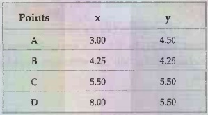
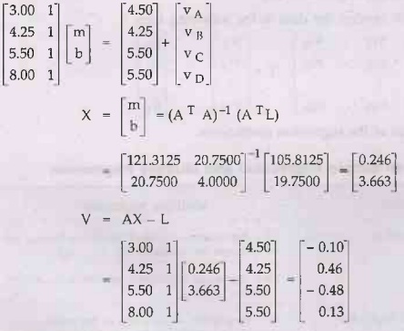
Solution:
Represent in matrix form:
Multiple Regression
•
Regression analysis is used to predict the value of
one or more responses from a set of predictors. It can also be used to estimate
the linear association between the predictors and responses. Predictors can be
continuous or categorical or a mixture ben of both.
•
If multiple independent variables affect the response
variable, then the analysis calls for a model different from that used for the
single predictor variable. In a situation where more than one independent
factor (variable) affects the outcome of process, a multiple regression model
is used. This is referred to as multiple linear regression model or multivariate
least squares fitting.
•
Let z1 ; z2;:::; zt,
be a set of r predictors believed to be related to a response variable Y. The
linear regression model for the jth sample unit has the form
Yj = β0
+ β1 zj1 + β2 zj2 + ... + βr
Zjr + εj
where
ε is a random error and β1,i= 0, 1, ..., r are un-known regression
coefficients.
•
With n independent observations, we can write one
model for each sample unit so that the model is now
Y =
Zβ + ε
where
Y is n × 1, Z is n × (r+1),β is (r+1)× 1 and ε is n × 1
•
In order to estimate ẞ, we take a least squares
approach that is analogous to what we did in the simple linear regression case.
• In matrix form, we can arrange the data in the following form:
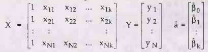
where βj are the estimates of the regression coefficients.
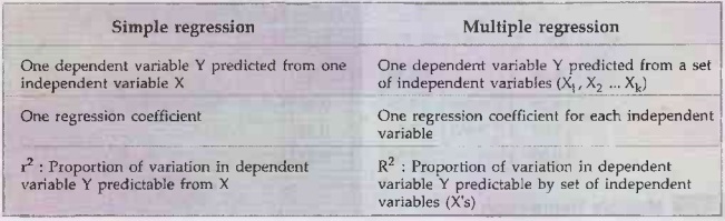
Difference between Simple Regression and Multiple Regression
Bayesian Linear Regression
•
Bayesian linear regression allows a useful mechanism
to deal with insufficient data, or poor distributed data. It allows user to put
a prior on the coefficients and on the noise so that in the absence of data,
the priors can take over. A prior is a distribution on a parameter.
•
If we could flip the coin an infinite number of
times, inferring its bias would be easy by the law of large numbers. However,
what if we could only flip the coin a handful of times? Would we guess that a
coin is biased if we saw three heads in three flips, an event that happens one
out of eight times with unbiased coins? The MLE would overfit these data,
inferring a coin bias of p =1.
•
A Bayesian approach avoids overfitting by quantifying
our prior knowledge that most coins are unbiased, that the prior on the bias
parameter is peaked around one-half. The data must overwhelm this prior
belief about coins.
•
Bayesian methods allow us to estimate model
parameters, to construct model forecasts and to conduct model comparisons.
Bayesian learning algorithms can calculate explicit probabilities for
hypotheses.
•
Bayesian classifiers use a simple idea that the
training data are utilized to calculate an observed probability of each class
based on feature values.
•
When Bayesian classifier is used for unclassified
data, it uses the observed probabilities to predict the most likely class for
the new features.
•
Each observed training example can incrementally
decrease or increase the estimated probability that a hypothesis is correct.
•
Prior knowledge can be combined with observed data to
determine the final probability of a hypothesis. In Bayesian learning, prior
knowledge is provided by asserting a prior probability for each candidate
hypotheses and a probability distribution over observed data for each possible
hypothesis.
•
Bayesian methods canaccommodate hypotheses that make
probabilistic predictions. New instances can be classified by combining the
predictions of multiple hypotheses, weighted by their probabilities.
•
Even in cases where Bayesian methods prove
computationally intractable, they can provide a standard of optimal decision
making against which other practical bus () methods can be measured.
•
Uses of Bayesian classifiers are as follows:
1.
Used in text-based classification for finding spam or junk mail filtering.
2.
Medical diagnosis.
3.
Network security such as detecting illegal intrusion.
•
The basic procedure for implementing Bayesian Linear
Regression is :
i)
Specify priors for the model parameter.
ii)
Create a model mapping the training inputs to the training outputs.
iii)
Have a Markov Chain Monte Carlo (MCMC) algorithm draw samples from the
posterior distributions for the parameters
Gradient Descent
•
Goal: Solving
minimization nonlinear problems through derivative information
•
First and second derivatives of the objective
function or the constraints play an important role in optimization. The first
order derivatives are called the gradient and the second order derivatives are
called the Hessian matrix.
•
Derivative based optimization is also called
nonlinear. Capable of determining search directions" according to an
objective function's derivative information.
•
Derivative based optimization methods are used for:
1.
Optimization of nonlinear neuro-fuzzy models
2.
Neural network learning
3.
Regression analysis in nonlinear models
•
Basic descent methods are as follows:
1.
Steepest descent
2.
Newton-Raphson method
Gradient
Descent:
•
Gradient descent is a first-order optimization
algorithm. To find a local minimum of a function using gradient descent, one
takes steps proportional to the negative of the gradient of the function at the
current point.
•
Gradient descent is popular for very large-scale
optimization problems because it is easy to implement, can handle black box
functions, and each iteration is cheap.
•
Given a differentiable scalar field f (x) and an
initial guess x1, gradient descent iteratively moves the guess
toward lower values of "f" by taking steps in the direction of the
negative gradient - ![]() f (x).
f (x).
•
Locally, the negated gradient is the steepest descent
direction, i.e., the direction that x would need to move in order to decrease
"f" the fastest. The algorithm typically converges to a local
minimum, but may rarely reach a saddle point, or not move at all if x1
lies at a local maximum.
•
The gradient will give the slope of the curve at that
x and its direction will point to an increase in the function. So we change x
in the opposite direction to lower the function value:
Xk+
1 = xk − λ![]() f (xk)
f (xk)
The
λ > 0 is a small number that forces the algorithm to make small jumps
Limitations
of Gradient Descent:
•
Gradient descent is relatively slow close to the
minimum technically, its asymptotic rate of convergence is inferior to many
other methods.
•
For poorly conditioned convex problems, gradient
descent increasingly 'zigzags' as the gradients point nearly orthogonally to
the shortest direction to a minimum point
Steepest
Descent:
•
Steepest descent is also known as gradient method.
•
This method is based on first order Taylor series
approximation of objective function. This method is also called saddle point
method. Fig. 8.3.5 shows steepest descent method.
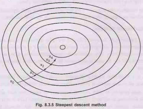
•
The Steepest Descent is the simplest of the gradient
methods. The choice of direction is where f decreases most quickly, which is in
the direction opposite to ![]() f (xi). The search starts at
an arbitrary point x0 and then go down the gradient, until reach close to the
solution.
f (xi). The search starts at
an arbitrary point x0 and then go down the gradient, until reach close to the
solution.
•
The method of steepest descent is the discrete
analogue of gradient descent, but the best move is computed using a local
minimization rather than computing a gradient. It is typically able to converge
in few steps but it is unable to escape local minima or plateaus in the
objective function.
•
The gradient is everywhere perpendicular to the
contour lines. After each line minimization the new gradient is always
orthogonal to the previous step direction. Consequently, the iterates tend to
zig-zag down the valley in a very manner.
•
The method of Steepest Descent is simple, easy to
apply, and each iteration is fast. It also very stable; if the minimum points
exist, the method is guaranteed to locate them after at least an infinite
number of iterations.
Artificial Intelligence and Machine Learning: Unit III: Supervised Learning : Tag: : Supervised Learning - Artificial Intelligence and Machine Learning - Regression
Related Topics
Related Subjects
Artificial Intelligence and Machine Learning
CS3491 4th Semester CSE/ECE Dept | 2021 Regulation | 4th Semester CSE/ECE Dept 2021 Regulation