Probabilistic Reasoning and Bayesian Networks

Probabilistic Reasoning and Bayesian Networks

The concept:

Probability based reasoning is the same as inferring directly from knowledge that can be given a probability rating based on the amount of uncertainty present. The uncertainties can arise from an inability to predict outcomes due to unreliable, vague incomplete or inconsistent knowledge. The probability of an uncertain event is a measure of the degree of likelihood of occurence of that event.

When one takes it for granted that certain parameters exist or known with certainty, solutions can be found out. Belief revision takes place whenever one encounters a piece of information that decreases the belief of the fact.

The source for all uncertainties is the real world. The following sources constitute the major causes of uncertainties -

i) Most information is not obtained personally but got from sources on which one has a lot of belief. Uncertainty prevails when the source does not send information in time or the information provided is not understood.

ii) In laboratory, experiments one takes it for granted that the equipment is properly calibrated and error free. If the equipment is faulty, the picture one gets about the situation is not correct which leads to uncertainty.

iii) Experimental errors like parallax errors are also sources of uncertainty.

iv) Imprecision in natural language is also a source of uncertainty.

v) A random event occurring is a major source of uncertainty.

vi) In judicial courts one may have seen or heard delivering judgements acquitting the accused for -

a) Lack of evidence

b) Lack of certainty in evidence thereby giving the benefit of doubt to the accused.

To handle these uncertain data, probability is the oldest technique available. Probabilistic reasoning is sometimes used when outcomes are unpredictable. For example, when a physician examines a patient, the patient's history, symptoms and test results provide some, but not conclusive evidence of possible ailments. This knowledge, together with the physician's experience with previous patients, improves the likelihood of predicting the unknown event, but there is still much uncertainty in most diagnoses.

One way to express confidence about such event is through probability. It is a mere number that expresses the chance of something happening or not happening.

Representing knowledge in uncertain domain:

Independence and conditional independence relationships among variables can greatly reduce the number of probabilities that need to be specified in order to define the full joint distribution. There is technique called as Bayesian Network which can be used to represent the dependencies among variables and to give a concise specification of any full joint probability distribution.

Bayesian Network

1. Definition

It is a data structure which is a graph, in which each node is annotated with quantitative probability information.

The nodes and edges in the graph are specified as follows:-

1) A set of random variables makes up the nodes of the network. Variables may be discrete or continuous.

2) A set of directed links or arrows connects pairs of nodes. If there is an arrow from node X to node Y, then X is said to be a parent of Y.

3) Each node Xi, has a conditional probability distribution P(X_i | Parents(X_i)) that quantifies the effect of the parents on the node.

4) The graph has no directed cycles (and hence is a directed, acyclic graph, or DAG).

The set of nodes and links is called as topology of the network. The topology of the network specifies the conditional independence relationships that hold in the domain.

The intutive meaning of an arrow between two nodes X and Y, in a properly constructed network, is that "X has direct influence on Y". The domain expert is a person who can identify such influence associations.

Once Bayesian network topology is specified then conditional probability distribution for each variable is specified. For specifying continuous probability distribution for a variable, its parent information is required.

The combination of topology and the conditional distributions is sufficient to specify the full joint distribution for all the variables.

Consider our example of simple world consisting of variables toothache, cavity, catch and weather. Weather is surly independent of other variables. Toothache and Catch are conditionally independent if given the information of cavity.

This relationships are represented by Bayesian network as shown below:

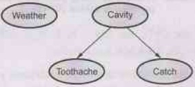
Fig. 7.3.1 A simple Bayesian network in which Weather is independent of other three variables and Toothache and Catch are conditionally independent, given the cavity

Note

1) The conditional independence of toothache and catch given the cavity is indicated by the absence of a link between toothache and catch.

2) The network represents the fact that cavity is a direct cause of toothache and catch.

3) No direct causal relationship exists between toothache and catch.

Consider another example of burglar alarm installed at A's home. This alarm notifies in case of burglary and can occasionally respond to minor earthquakes. There are two neighbours to A, M and J. M and J promised to call A in office when they hear alarm. J always calls A when he hears alarm, but many times he is confused between telephone ring and burglar alarm. M many a times misses alarm because he keeps on listening to loud music. Given the evidence of who has or has not called, we are to estimate the probability of burglary.

The Bayesian network for above problem along with the associated probabilities is shown below:

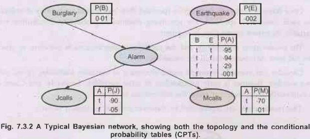
Note In the figure, in the CPTS, the letters B, E, A, J and M stand for Burglary, Earthquake, Alarm, Johncalls, Marycalls respectively.

1) In the figure, each distribution is shown as conditional probability table. Each row in the table contains the conditional probability of each node value for a 91 conditioning case. A conditioning case is just a possible combination of values for the parent nodes. Each row must sum upto 1 because the entries represent an exhaustive set of cases for the variable.

2) For boolean variable if it is true and its probability is know to be 'P' then when it is false its probability is 1-P and it is ommited from the table (because it can be deduced from 'P').

3) A table for a boolean variable with k boolean parents contains 2k independently specifiable probabilities. A node with no parents has only one row, representing the prior probabilities of each possible value of the variable.

2. The Semantics of Bayesian Networks

There are two ways through which semantic (meaning) of Bayesian network can be understood.

One way is to view network as a representation of the joint probability distribution. This view helps to constructs networks. Second way is to view a network as an encoding of a collection of conditional independence statements. This view helps in designing inference procedure semantically both views are equivalent.

Understanding semantic of Bayesian network method:

• Representing the full joint distribution:

1) Every entry in the full joint probability distribution (hereafter abbreviated as "joint") can be calculated from the information in the network.

2) A generic entry in the joint distribution is the probability of a conjunction of particular assignments to each variable, such as P(X₁ = x₁ ^.....^x_n = x_n)

follg3) The notation P(x₁,...,x_n) is used as an abbrevation for this.

4) The value of this entry is given by the formula.

P(x₁,...,x_n) = Пⁿ_j=1 P(x_i | parents (X_i))                          ……(7.3.1)

where parents (x_i) denotes the specific values of the variables in parents (x_i).

5) Thus, each entry in the joint distribution is represented by the product of the appropriate elements of the Conditional Probability Tables (CPTs) in the Bayesian network. The CPTs therefore, provide a decomposed representation of the joint distribution.

We can calculate the probability that the alarm has sounded, but neither a burglary nor an earthquake has occurred and both J and M call. We use single letter names for the variables:

P(j Ʌ m Ʌ a Ʌ⌐ b Ʌ⌐ e) = P(j | a) P(m | a) P(a |⌐ b Ʌ⌐ e) P(⌐ b) P(⌐e)

= 0.90 × 0.70 × 0.001 × 0.999 x 0.998 = 0.00062

6) Remember that the full joint distribution can be used to answer any query about the domain.

If a Bayesian network is a representation of the joint distribution, then it too can be used to answer any query, by summing all the relevant joint entries. A method for constructing Bayesian network:

1) We rewrite the joint distribution in terms of a conditional probability, using the product rule.

P(x₁,...,x_n) = P(x_n | X_n-1,...,X₁) P(x_n-1,...,x₁).

2) Then the process is represented, reducing each conjunctive probability to a conditional probability and a smaller conjunction. We end up with one bigproduct.

P(x₁,...,x_n) = P(x_n | x_n-1,..., x₁)P(x_n-1 x_n-2 ,...,x₁).....P(x₂ | x₁) P(x₁)

= IIⁿ_i=1 P(x_i | x_j-1,….x₁)                                      …..(7.3.2)

3) Above identity holds true for any set of random variables and is called the Chain rule. Comparing it with equation (7.3.1). We see that the specification of the joint distribution is equivalent to the general assertion that, for every variable X_i in the network,

P(X_i X_i-1,....X₁) = P(X_i | Parents(X_j)),

provided that parents (X_i) (X_i-1,....X₁}. This last condition is satisfied by labeling the nodes in any order that is consistent with the partial order implicit in the graph structure.

4) Bayesian network is correct representation of the domain only if each node is conditionally independent of its predecessors in the node ordering, given its parents.

5) In order to construct a Bayesian network with the correct structure for the domain, we need to choose parents for each node such that this property holds. Intuitively, the parents of node X; should contain all those nodes in X_i,....X_i-1 that directly influence X_i.

For example: Suppose we have completed the network in Fig. 7.2.2 except for the choice of parents for M calls, M calls is certainly influenced by whether there is a burglary or an earthquake, but not directly influenced. Intitutively, our knowledge of the domain tells us that these events influence M's calling behaviour only through their effect on the alarm. Also given the state of the alarm, whether J calls has no influence on M's calling. Formally speaking, we believe that the following conditional independence statement holds:

P(M Calls |J Calls, Alarm, Earthquake, Burglary) = P(M calls | Alarm).

• Compactness and node ordering:

Bayesian network are compact and they possess a property of being locally structured (also called as sparse systems). In a locally structured system, each sub component interacts directly with only a bounded number of other components, regardless of the total number of components.

⇒ Local structure is usually associated with linear rather than exponential growth in complexity.

⇒ We assume 'n' boolean variables for simplicity, then the amount of information on needed to specify each conditional probability table will be at most 2k numbers. Where each random variable is influenced by 'k' other variables.

⇒ The complete network can be specified by n2^k numbers.

With some values of 'n' the joint distribution contains 2ⁿ numbers.

⇒ To make this concrete, suppose we have n = 30 nodes, each with five parents (k=5). Then the Bayesian network requires 960 numbers, but the full joint distribution requires over a billion.

Ordering of nodes in Bayesian network:

1) The correct order in which to add nodes is to add the "root causes" first, then the variables they influence, and so on, until we reach the "leaves", which have no direct causal influence on the other variables.

2) If wrong order is choosen we get more complicated network.

For example: Consider network shown in following diagram.

The network construction process goes as follows:

i) Adding M calls: No parent.

ii) Adding J calls: If M calls, that probably means the alarm has gone off, which ofcourse would make it more likely that J calls. Therefore J calls needs M calls as a parent.

iii) Adding alarm: Clearly, if both call, it is more likely that the alarm has gone off than if just one or neither call, so we need both M calls and J calls as parent.

iv) Adding burglary: If we know the alarm state, then the call from J or M might give us information about phone ringing or M's music, but not about burglary : P(Burglary Alarm, J calls, M calls) = P(Burglary | Alarm).

Hence we need just alarm as parent.

v) Adding earthquake: If the alarm is on, it is more likely that there has been an 2 earthquake. (The alarm is an earthquake detector of sorts). But if we know that there has been a burglary, then that explains the alarm, and the probability of an earthquake would be only slightly above normal. Hence, we need both Alarm and Burglary as parents. The network is shown below.

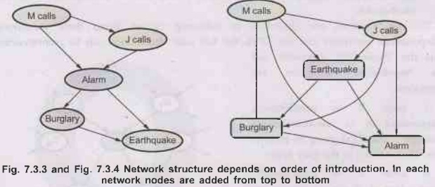
• Consider example of a very bad node ordering as shown in the Fig. 7.2.4: M calls, J calls, Earthquake, Burglary, Alarm are nodes. This network requires 31 distinct probabilities to be specified exactly the same as the full joint distribution. It is important to realize, however, that any of the three networks can represent exactly the same joint distribution. The last two versions simply fail to represent all conditional independence relationships and hence end up specifying a lot of unnecessary numbers instead.

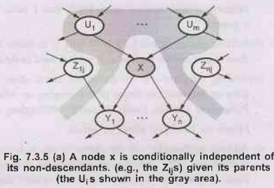
3. Conditional Independence Relations in Bayesian Networks

One can start from a "topological" semantics that specifies the conditional independence relationships encoded by the graph structure, and from these we can derive the "numerical" semantics. The topological semantics is given by either of the following specifications, which are equivalent.

1) A node is conditionally independent of its non-descendants, given its parents. For example, in Fig. 7.3.2 J calls is independent of Burglary and Earthquake, given the value of Alarm.

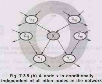
2) A node is conditionally independent of all other nodes in the network, given it’s parents, children, and children’s parents- that is, given its Markov blanket.

For example: Burglary is independent of J calls and M calls given Alarm and Earthquake.

This specifications are illustrated in following figures. From these conditional independence assertions and the CPTs, the full joint distribution can be reconstructed; thus the "numerical" semantics and the "topological" semantics are equivalent.

A node X is conditionally independent of its non-descendants (example - - The Z1js) given its parents(the U; is shown in the gray area).

As node X is conditionally on independent of all other nodes in the network given its Markove blanket (the gray area).

Efficient representation of conditional representation:

If the maximum number of parents k is smallish, filling in the CPT for a node, would require up to O(2^k) numbers.

To avoid this big relationship number canconical distribution is used. In this a complete table is specified by naming the patterns supplied with parameters, which can describe relationship which are necessary. A deterministic node represents canonical distribution. A deterministic node is a node whose value is exactly specified by the value of its parents with no uncertainity.

The uncertain relationships are often represented by noisy-OR relationships. [Noisy-OR is generalization of logical OR]. The noisy-OR model allows uncertainity about the parent to cause the child to be true i.e. the causal relationship between parent and child would be inhibited.

For example: A patient could have cold (parent) but not exhibit a fever (child).

For noisy-OR model it is required that all the possible effects of parent must be listed. It should be clear that inhibition of one parent is independent of other parent.

The Hybrid Bayesian Network

A network with both discrete and continuous variables is called as hybrid Bayesian network. For representing continuous variable its discretization is done in terms of intervals (because it can have infinite values).

To specify a hybrid network, we have to specify two new kinds of distributions. The conditional distribution for a continuous variable given discrete or continuous parents; and the conditional distribution for a discrete variable given continuous parents.

Consider the simple example in following diagram, in which a customer buys some fruit depending on its cost, which depends in turn on the size of the harvest and whether the government's subsidy scheme is operating. The variable Cost is continuous

and has continuous and discrete parents; the variable Buys is discrete and has a continuous parent.

For the cost variable, we need to specify P(Cost Harvest, Subsidy). The discrete parent is handled by explicit enumeration that is, specifying both P(Cost | Harvest, Subsidy) and P(Cost Harvest, Subsidy). To handle Harvest, we specify how the distribution over the cost 'c' depends on the continuous value 'h', of Harvest. In other words, we specify the parameter of the cost distribution as a function of 'h'.

Inferencing in Bayesian Networks

1. Exact Inference in Bayesian Networks

For inferencing in probabilistic system, it is required to calculate posterior probability distribution for a set of query variables, where some observed events are given. [That is we have some values attached to evidence variables].

• Notation Revisited:

The notation used in inferencing is same as the one used in probability theory.

X: Query variable.

E: The set of evidence variables E₁,....., E_m and 'e' is the perticular observed event. Y: The set of non-evidence variables Y₁, Y₂,..... Y_k [Non-evidence variables are also called as hidden variables].

X: It the complete set of all the types of variables, where X = {X} U E U Y.

• Generally the query requires the posterior probability distribution P(X | e) [assuming that query variable is not among the evidence variables, if it is, then posterior distribution for X simply gives probability 1 to the observed value]. [Note that query can contain more than one variable. For study purpose we are assuming single variable].

• Example: In the burglary case, if the observed event is Jcalls = true and Mcalls true.

The query is 'Has burglary occured?'

The probability distribution for this situation would be,

P(Burglary | J calls = true, M calls = true) = < 0.284, 0.716 >

2. Inference by Enumeration

A Bayesian network gives a complete representation of the full joint distribution. These full joint distributions can be written as product of conditional probabilities from the Bayesian network.

A query can be answered using Bayesian network by computing sums of products of conditional probabilities from the network.

• The algorithm

The algorithm ENUMERATE-JOINT-ASK gives inference by enumerating on full joint distribution.

Characteristics of algorithm:

1) It takes input a full joint distribution P and looks up values in it. [The same algorithm can be modified to take input as Bayesian network and looking up in joint entries by multiplying the corresponding conditional probability table entries from Bayesian network.

2) The ENUMERATION-JOINT-ASK uses ENUMERATION-ASK (EA) algorithm which evaluate expression using depth-first recursions. Therefore, the space complexity of EA is only linear in the number of variables. The algorithm sums over the full joint distribution without ever constructing it explicitely. The time complexity for network with 'n' boolean variables is always O(2ⁿ) which is better than the O(n 2ⁿ) required in simple inferencing approach (using posterior probability).

3) The drawback of the algorithm is, it keeps on evaluating repeated sub expression which results in wastage of computation time.

The enumeration algorithm for answering queries on Bayesian network.

• The algorithm

Function ENUMERATION-ASK (X, e, bn) returns a distribution over X.

Inputs: X, the query variable

e, observed values for variables E.

bn, a Bayes net with variables {X} UEU Y/* y = Hidden variable */

Q(X) ← A distribution over X, initially empty for each value x_i of X do extend e with value x_i for X.

Q(x_i) ← ENUMERATE-ALL (VARS[bn] e) return NORMALIZE (Q(x)).

Function ENUMERATE-ALL (vars, e) returns a real number.

if EMPTY? (vars) then return 1.0

Y ← FIRST (vars)

If Y has value y in e.

Then return P(y | parents (Y)) X ENUMERATE-ALL (REST(vars), e)

else return, Σ_y Ply parents (Y)) X ENUMERATE-ALL (REST(vars), ey)

where e_yis e extended with Y = y.

Example:

Consider query,

P(Burglary | J calls = true, M calls =true)

Hidden variables in the queries are → Earthquake and Alarm.

using the query equation.

P(Burglary | j, m) = α P( Burglary, J, M) = α Σ_e Σ_a P(Burglary, e, a, j, m)

The semantics of Bayesian networks (equation 7.2.1) then gives us an expression in terms of CPT entries. For simplicity, we will do this just for Burglary = true.

P(b | j, m) = α Σ_e Σ_aP(b)P(e)P(a | b, e)P(j | a) P(m | a)

• To compute this expression, we have to add four terms, each computed by multiplying five numbers.

• Worst case, where we have to sum out almost all the variables, the complexity of the algorithm for a network with n boolean variables is O(n2ⁿ).

• An improvement can be obtained from the following simple observations. The P(b) term is a constant and can be moved outside the summations over a and e, and the P(e) term can be moved outside the summation over a. Hence, we have

P(b | j, m) = α P(b) Σ_e P(e) Σ_aP(a | b, e)P(j | a) P(m, a)

This expression can be evaluated by looping through the variables in order, multiplying CPT entries as we go. For each summation, we also need to loop over the variable's possible values. The structure of this computation is shown in following diagram. Using the numbers from Fig. 7.3.2, we obtain P(b | j, m) = α × 0.00059224. The corresponding computation for ⌐b yields α × 0.0014919;

Hence,

P(B | j, m)= α < 0.00059224, 0.0014919 >

≈ <0.284, 0.716 >

That is, the chance of burglary, given calls from both neighbours is about 28 %. Note In the Fig. 7.3.7, the evalution proceeds top to down, multiplying values along each path and summing at the "t" nodes. Observe that there is repetition of paths for j and m.

3. The Variable Elimination Algorithm

The enumeration algorithm can be improved substantially by eliminating calculations of repeated sub expression in tree. Calculation can be done once and save the results for later use. This is a form of dynamic programming.

Working of variable elimination algorithm

1) It works by evaluating expressions such as [P(b | j, m) = α P(b) Σ_e P(e) Σ_a P(a | b, e) P(j | a) P(m | a)] in right-to-left order.

2) Intermediate results are stored and summations over each variable are done only for those portions of the expression that depends on the variable.

For example: Consider the Burglary network.

We evaluate the expression:

3) Factors: Each part of the expression is annotated with the name of the associated variable, these parts are called factors.

Steps in algorithm:

i) The factor for M, P (m | a), does not require summing over M. Probability is stored, given each value of a, in a two-element factor,

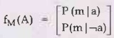
Note f_M means that M was used to produce f.

ii) Store the factor for J as the two-element vector f_j (A).

iii) The factor for A is P(a | B, e) which will be a 2×2×2 matrix f_A (A, B, E).

iv) Summing out A from the product of these tree factors. This will give 2×2 matrix whose indices range over just B and E. We put bar over A in the name of the matrix to indicate that A has been summed out.

F_ȂJM(B, E) =Σ_a f_A (a, B, E) × f_j (a) × f_M (a)

= f_A (a, B, E) x f_J(a) x f_M (a) + f_A ( ⌐a, B, E) x f_j (¬a)×f_m (¬a)

The multiplication process used is called a printwise product.

v) Processing E in the same way (i.e.) sum out E from the product of

f_E (E) and f_ȂJM (B, E):

f_ȂJM (B) = f_E (e) × f_ȂJM (B, e) + f_E (¬e) × f_ȂJM (B, ¬e).

vi) Compute the answer simply by multiplying the factor for B. (i.e.) (f_B|B) = P(B), 701 by the accumulated matrix (B) :

P(B | j, m) =  α f_B (B) x f _EȂJM (B).

From the above sequence of steps it can be noticed that two computational operations are required.

a) Pointwise product of a pair of factors.

b) Summing out a variable from a product of factors.

a) Pointwise product of a pair of factors: The pointwise product of two factors f₁ and f₂ yields a new factor f, those variables are the union of the variables in f₁ and f₂. Suppose the two factors have variables Y₁,..., Y_k. Then we have f(x₁,..., X_j, Y₁,.... Y_k, Z₁,.....Z_l) = f₁ (X₁,....X_j, Y₁.... Y_k) f₂(Y₁,..... Y_k, Z₁,....Z_l). If all the variables are binary, then f₁ and f₂ have 2^j+k and 2^k+l entries and the pointwise product has 2^j+k+1 entries.

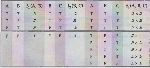
For example: Given two factors f₁ (A, B) and f₂ (B, C) with probability distributions shown below, the pointwise product f₁ × f₂ is given as f₁ (A, B, C).

b) Summing out a variable from a product of factors: It is a straight forward computation. Any factor that does not depend on the variable to be summed out can be moved outside the summation process.

For example:

Σ_e f_E (e) × f_A (A, B, e) × f_j (A) × f_M (A) = f_j (A) × f_M (A) × Σ e f_E (e) × f_A (A, B, e). Now, the pointwise product inside the summation is computed and the variable is summed out of the resulting matrix.

F_j (A) × f_M (A) × Σ_e f_E (e) × f_A (A, B, e) = f_j (A) × f_M (A) × f_EA(A, B).

Matrices are not multiplied until we need to sum but a variable from the accumulated product. At that point, multiply those matrices that include the variable to be summed out.

The procedure for pointwise product and summing is given below, the variable elimination algorithm is shown below:

Function ELIMINATION-ASK (X, e, bn) returns a distribution over X

Inputs: X, the query variable

e, evidence specified as an event

bn, a Bayesian network specifying joint distribution P(X₁,..., X_n).

Factors ← [ ] : vars ← REVERSE (VARS [bn])

for each var in vars do

Factors ←[MAKE-FACTOR (var, e) factors]

if var is a hidden variable then

Factors←SUM-OUT (var, factors)

returns NORMALIZE (POINTWISE-PRODUCT (factors)).

P (J calls, Burglary = True)

The first step is to write out the nested summation.

P(J | b) = α P(b) Σ_e P(e) Σ_a P(a | b, e) P(J | a) Σ_m P(M | a).

Evaluating this expression from right to left,

Σ_m P(M | a) is equal to 1.

Note The variable M is irrelevant to this query. Result of the query P (J calls/Burglary = True) is unchanged if we remove M calls from the network. We can remove any leaf node which is not a query variable or an evidence variable. After its removal, there may be more leaf nodes and they may be irrelevant. Eventually we find that every variable that is not an ancestor of a query variable or evidence variable is, irrelevant to the query. A variable elimination algorithm can remove all these variables before evaluating the query.

4. The Complexity Involved in Exact Inferencing

The variable elimination algorithm is more efficient than enumeration algorithm because it avoids repeated computations as well as drops irrelevant variables.

The variable elimination algorithm constructs the factor, deriving its operation. The space and time complexity of variable elimination is directly dependant on size of the largest factor constructed during the operation. Basically the factor construction is determined by the order of elimination of variables and by the structure of the network; which affects both space and time complexity.

For developing more efficient process we can construct singly connected networks which are also called as polytrees. In singly connected network, there is at most one undirected path between any two nodes in the networks. The singly connected networks have property that, the time and space complexity of exact inference in polytrees is linear in the size of the network. Here the size is defined as the number of CPT entries. If the number of parents of each node is bounded by a constant, then the complexity I will also be linear in the number of nodes.

For example: The Burglary network shown in the Fig. 7.3.2 is a polytrees.

[Note that every problem may not be represented as polytrees].

In multiply networks [In this, their can be multiple undirected paths between any two nodes and more than one directed path between some pair of nodes], variable elimination takes exponential time and space complexity in the worst case, even when the number of parents per node is bounded. It should be noted that variable elimination includes inference in propositional logic as a special case and inference in Bayesian network is NP-hard. In fact it is strictly harder than NP-complete problem.

Clustering algorithm:

1) Clustering algorithm (known as joint tree algorithms) in which inferencing time can be reduced to O(n). In clustering individual nodes of the network are joint to form cluster nodes to such a way that the resulting network is a polytree.

2) The variable elimination algorithm is efficient algorithm for answering individual queries. Posterior probabilities are computed for all the variables in the network. It can be less efficient, in polytree network because it needs to issue O(n) queries costing O(n) each, for a total of O(n²) time, clustering algorithm, improves over it.

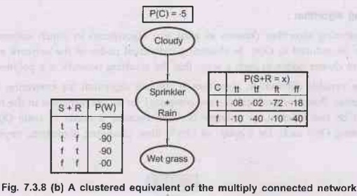
For example: The multiply connected network shown in Fig. 7.3.8 (a) can be converted into a polytree by combining the Sprinkler and Rain node into a clusternode called Sprinkler + Rain, as shown in Fig. 7.2.8 (b). The two Boolean nodes are replaced by a meganode that takes on four possible values: TT, TF, FT, FF. The meganode has only one parent, the Boolean variable. Cloudy, so there are two conditioning cases.

Peculiarities of algorithm:

1) Once the network is in polytree form, a special-purpose inference algorithm is applied. Essentially, the algorithm is a form of constraint propagation where the constraints ensure that neighbouring clusters agree on the posterior probability of any variables that they have in common.

2) With careful book keeping, this algorithm is able to compute posterior probabilities for all the non-evidence nodes in the network in time O(n), where n is now the size of the modified network.

3) However, the NP-hardness of the problem continues: if a network requires exponential time and space with variable elimination, then the CPTs in the clustered network will require exponential time and space to construct.

Approximate Inference in Bayesian Network

Because of the fact that exact inference in multiply connected network is intractable problem, we go for approximate inferencing.

For approximate inferencing randomize sampling algorithm (Monte Carlo Algorithm) is used. Its accuracy depends on number of samples generated. Monte Carlo Algorithm is widely used in problem areas where it is difficult to calculate exact quantities.

There are two families of Monte Carlo algorithm:

1) Direct sampling algorithm.

2) Markov chain sampling algorithm.

1. Direct Sampling Algorithm

1) The basic element in any sampling algorithm is the generation of samples from a known probability distribution.

For example: An unbiased coin can be thought of as a random variable coin with values (heads, tails) and a prior distribution P(coin) <0.5, 0.5>. Sampling from this distribution is exactly like flipping the coin: with probability 0.5 it will return 9879 heads, and with probability 0.5 it will return tails. Given a source of random numbers in the range [0, 1], it is a simple matter to sample any distribution on a single variable.

2) The simplest kind of random sampling process for Bayesian networks generates events from a network that has no evidence associated with it. The idea is to sample each variable in turn, in topological order.

3) The probability distribution from which the value is sampled is conditioned on the values already assigned to the variable's parents.

4) The sampling algorithm:

Function PRIOR-SAMPLE (bn) returns an event sampled from the prior specified by bn.

inputs: bn, a Bayesian network specifying joint distribution P(X₁,..., X_n).

X ← an event with n elements.

for i = 1 to n do

x_i ← a random sample from P(X_i parent (X_i))

return x.

5) Applying operations of algorithm on the network in Fig. 7.3.8 (a) assuming an ordering [Cloudy, Sprinkler, Rain, WetGrass]:

i) Sample from P(Cloudy) = <0.5, 0.5>; suppose this returns true.

ii) Sample from P(Sprinkler | Cloudy = true) = <0.1, 0.9>; suppose this returns false.

iii) Sample from P(Rain | Cloudy = true) = <0.8, 0.2>; suppose this returns true. iv) Sample from P(WetGrass | Sprinkler = false, Rain = true) <0.9, 0.1>; suppose this returns true.

In this case PRIOR-SAMPLE returns the event [true, false, true, true].

6) PRIOR-SAMPLE generates samples from the prior joint distribution specified by the nework. First, let S_ps (x₁,...,x_n) be the probability that a specific event is generated by the PRIOR-SAMPLE algorithm. Just looking at the sampling process, we have,

S_ps (x₁,...,x_n)= Πⁿ_i=1 P(x_i | parents(X_i)).

Because each sampling step depends only on the parent values. This expression is also the probability of the event according to the Bayesian net's representation of the joint distribution. We have,

S_ps (x₁,...,x_n) = P(x₁,...,x_n)

7) In any sampling algorithm, the answers are computed by counting the actual samples generated. Suppose there are N total samples, and let N (x₁,...,x_n) be the frequency of the specific event x₁,...,x_n. We expect this frequency to converge in the limit, to its expected value according to the sampling probability:-

N → ^lim ∞ N_ps (x_1, …., x_n )/N = S_ps (x_{1, …,} x_n) = P(x₁,….x_n)         ... (7.3.4)

For example: Consider the event produced earlier : [true, false, true, true]. The b. a sampling probability for this event is,

S_ps (true, false, true, true) = 0.5 × 0.9 × 0.8 × 0.9

= 0.324

Hence, in the limit of large N, we expect 32.4 % of the samples to be of this event.

8) Whenever we use an approximate equality ("≈"), we mean it in exactly this sense that the estimated probability becomes exact in the large sample limit. Such an estimate is called consistent.

For example: One can produce a consistent estimate of the probability of any partially specified event x₁,...,x_n, where m≤n, as follows: -

P(x₁,...,x_m) ≈ N_ps (x₁,...,x_m)/N                                     ….(7.3.5)

That is, the probability of the event can be estimated as the fraction of all complete events generated by the sampling process that match the partially specified event.

For example: If we generate 1000 samples from the sprinkler network, and 511 of them have, Rain = true, then the estimated probability of rain, written as P(Rain = true), is 0.511.

2. Rejection Sampling in Bayesian Networks

1) Rejection sampling is a method for producing samples from a hard-to-sample distribution given an easy-to-simple distribution.

2) It can be used to compute conditional probabilities; that is, to determine P(X | e).

3) The Rejection Sampling algorithm is,

function REJECTION-SAMPLING (x, e, bn, N) returns an estimate of P(X | e)

inputs: X, the query variable

e, evidence specified as an event.

bn, a Bayesian network.

N, the total number of samples to be generated.

local variables: N, a vector of counts over X, initially zero.

for j = 1 to N do

X ←PRIOR-SAMPLE (bn)

if X is consistent with e is N[x] ← N[x] +1 where x is the value of  X in x.

return NORMALIZE (N[x]).

The rejection sampling algorithm for answering queries given evidence in a Bayesian network.

• Working of algorithm:

i) It generates samples from the prior distribution specified by the network.

ii) It rejects all those samples that do not match the evidence.

iii) Finally, the estimate P(X = x | e) is obtained by counting how often X = x occurs in the remaining samples.

4) Let P(X | e) be the estimated distribution that the algorithm returns. From the definition of the algorithm, we have,

P(X | e) = α N_ps (X, e) = N_ps (X, e)/N_ps (e)

from equation (7.3.5) this becomes,

P(X | e) ≈ P(x, e)/P(e) = P(x, e).

That is, rejection sampling produces a consistent estimate of the rule probability. 5) Applying operations of algorithm on the network in the Fig. 7.3.8 (a), let us assume that we wish to estimate P (Rain/Sprinkler = true), using 100 samples. Of the 100 that we generate, suppose 8 have Rain = true and 19 have Rain = false. Hence,

P(Rain | Sprinkler = true) ≈NORMALIZE

(<8.19>) = <0.296, 0.704 >

The true answer is <0.3, 0.7>

6) As more samples are collected, the estimate will converges to the true answer. The standard deviation of the error in each probability will be proportional to 1/√n, where 'n' is the number of samples used in the estimate.

7) The biggest problem with rejection sampling is that it rejects so many samples ! The fraction of samples consistent with the evidence 'e' drops exponentially as the number of evidence variables grows, so the procedure is simply unusable for complex problems.

3. Likelihood Weighing in Bayesian Network

1) Likelihood weighing avoids the inefficiency of rejection sampling by generating only events that are consistent with the evidence 'e'.

2) The Likelihood Weighing algorithm is,

Function LIKELIHOOD-WEIGHING (X, e, bn, N) returns an estimate of P(X | e) inputs: X, the query variable

e, evidence specified as an event

bn, a Bayesian network.

N, the total number of samples to be generated.

Local variables: W, a vector of weighted counts over X, initially zero.

for j = 1 to N do

X, w← WEIGHTED-SAMPLE (bn)

W[X]← W[x] + w where x is the value of X in x.

return NORMALIZE (W[X]).

Function WEIGHTED-SAMPLE (bn, e) returns an event and a weight

X ← an event with n elements; w← 1.

for i = 1 to n do

if X, has a value x_i in e

then w ← wX P(X_i = x_i parents(X_i))

else x_i ← a random sample from P(X_i | parents (X_i))

return X, w.

Note on likelihood weighing algorithm -

i) It fixes the values for the evidence variables E and samples only the remaining variables X and Y. This guarantees that each event generated is consistent with the evidence.

ii) Not all events are equal, however, before tallying the counts in the distribution for the query variable, each event is weighted by the likelihood that the event 19 accords to the evidence, as measured by the product of the conditional of probabilities for each evidence variable, given its parents.

iii) Intuitively, events in which the actual evidence appears unlikely should be given less weight.

3) Applying operations of algorithm on the network Fig. 7.3.8 (a), with the query P(Rain/Sprinkler = true, WetGrass = true). The process goes as follows:

i) The weight w is set to 1.0

ii) Now, an event is generated.

• Sample from P(Cloudy) = <0.5, 0.5>; suppose this returns true.

• Sprinkler is an evidence variable with value true. Therefore, we set

w ← w P (Sprinkler = true | Cloudy = true) = 0.1.

• Sample from P(Rain | Cloudy = true) = <0.8, 0.2>; suppose this returns true.

• WetGrass is an evidence variable with value true. Therefore, we set

W ← w P(Wet Grass = true | Sprinkler = true, Rain = true) = 0.099.

iii) Here WEIGHTED-SAMPLE returns the event [true, true, true, true] with weight 0.099, and this is tallied under Rain = true.

iv) The weight is low because the event describes a cloudy day, which makes the sprinkler unlikely to be on.

4) Likelihood Weighting working:

i)Examine the sampling distribution S_ws for WEIGHTED-SAMPLE.

ii) The evidence variables E are fixed with values 'e'.

iii) Call the other variables Z, that is, Z = {X}U Y.

iv) The algorithm samples each variable in Z, in given its parent values:

S_ws (Z, e) =II^l_i=1 P(Z_i | parents (Z_i))... (7.3.6)

Notice that Parents (Z_i) can include both hidden variables and evidence variables. Unlike the prior distribution P(Z), the distribution S_ws pays some attention to the son evidence the sampled values for each Z_i will be influenced by evidence among Z_i's ancestors.

v) On the other hand, S_ws pays less attention to the evidence than does the true Som posterior distribution P(Z | e), because the sampled values for each Z_i ignore evidence among Z_i's non ancestors.

vi) The likelihood weight w makes up for the difference between the actual and desired sampling distribution. The weight for a given sample 'x', composed from Z and 'e', is the product of the likelihood for each evidence variable given its parents (some or all of which may be among the Z_is):

w(Z, e) = II^m_j=l P(e_i / parents(E_i)                              .... (7.3.7)

vii) Multiplying equations (7.3.4) and (7.3.5), we see that the weighted probability of a sample has the particularly convenient form,

S_ws (Z, e) W(Z, e) = Π^l_i=1 P(y_i | parents(Y_i))

Π^m_i=1 P(e_i | parents(E_i)) = P(y, e)

Because the two products cover all the variables in the network, allowing us to use equation (7.3.1) for the joint probability.

viii) It can be easy to show that likelihood weighting estimates are consistent. For any particular value x of X, the estimated posterior probability can be calculated as follows:

P(x | e) =α Σ_y N_ws (x, y, e) w (x, y, e)

from LIKELIHOOD-WEIGHTING.

 = α՛ Σ_y S_ws (x, y, e) w (x, y, e)

from large N.

= α' Σ_y Ρ(x, y, e)

= α' P(x, e) =P(x | e)by equation (7.3.8)

Hence, likelihood weighting returns consistent estimates.

5) Performance of algorithm:

i) Likelihood weighting uses all the samples generated therefore it can be much more efficient than rejection sampling.

ii) It will, suffer a degradation in performance as the number of evidence variables increases.

iii) Because most samples will have very low weights and hence the weighted estimate will be dominated by the tiny fraction of samples that accord more than an infinitesimal likelihood to the evidence.

iv) The problem is exacerbated if the evidence variables occur late in the variable ordering, because then the samples will be the simulations that bear little resemblance to the reality suggested by the evidence.

4. Markov Chain Monte Carlo (MCMC) Algorithm for Inference in Bayesian Networks

Working of MCMC algorithm

1) MCMC generates each event by making a random change to the preceding event. It is therefore helpful to think of the network as being in a particular current state specifying a value for every variable.

2) The next state is generated by randomly sampling a value for one of the non- evidence variables X_i, conditioned on the current values of the variables in the Markov blanket of X_i.

3) MCMC therefore wonders randomly around the state space - the space of possible complete assignments flipping one variable at a time, but keeping the evidence variables fixed.

4) For example: Consider the query P(rain | Sprinkler = true, WetGrass = true) applied to the network of Fig. 7.3.8 (a). The evidence variables 'Sprinkler' and 'WetGrass' are fixed to their observed values and the hidden variables 'Cloudy'and 'Rain' are initialized randomly. Let us say to true and false respectively. Thus, the initial state is [true, true, false, true]. Now the following steps are executed repeatedly:

a) Cloudy is sampled, given the current values of its Markov blanket variables : in this case, we sample from P(Cloudy | Sprinkler = true, Rain = false), (Shortly we will show how to calculate this distribution). Suppose the result is y = false. Then the new current state is [false, true, false, true].

b) Rain is sampled, given the current values of its Markov blanket variables : In this case we sample from P(Rain Cloudy false, Sprinkler = true, WetGrass = true). Suppose this yields Rain = true. The new current state is [false, true, true, true].

5) Each state visited during this process is a sample that contributes to the estimate, for the query variable Rain. If the process visits 20 states where Rain is true and 60 states where Rain is false, then the answer to the query is NORMALIZE (<20, 60>) = <0.25, 0.75>).

6) The complete algorithm is shown as follows:-

Function MCMC-ASK (X, e, bn, N) returns an estimate of P(X | e)

local variables: N[X], a vector of counts over X, initially zero.

Z, the nonevidence variables in bn.

X, the current state of the network, initially copied from e.

initialize X with random values for the variables in Z.

for j = 1 to N do

N[x] ←N[x] +1 where x is the value of X in x.

for each Z_i in Z do...

sample the value of Z_i in X from P(Z_i |mb(Z_i)) given the value of MB (Z_i) in X return NORMALIZE (N[X]).

Why MCMC works

1) It should be noticed that the sampling process settles into a "dynamic equilibrium" in which the long-run fraction of time spent in each state is exactly proporitional to its posterior probability.

2) This remarkable property follows from the specific transition probability with which the process moves from one state to another, as defined by the conditional distribution given the Markov blanket of the variable being sampled.

3) Let q(X →X') be the probability that the process makes a transition from state X to X'. This transition probability defines what is called a Markov chain on the state space.

4) Now suppose that we run the Markov chain for 't' steps, and let л(X) be the probability that the system is in state X at time 't'.

- Similarly, let л_t+1(X') be the probability of being in state X' at time 't+1.'

- Given л_t (X)

- We can calculate л_t+1(X') by summing for all states the system could be in at time 't'.

- The probability of being in that state is the times the probability of making the transition to X' →π_t+1(X') = Σ_x π_t (X) q(X→X')

5) We will say that the chain has reached its stationary distribution if л_t = π_t+1. Call this stationary distribution л; its defining equation is therefore,

π (X') = Σ_X π (X) q (X→X') for all X'                                 …..(7.3.9)

Under certain standard assumptions about the transition probability distribution there is exactly one distribution л satisfying this equation for any given q.

6) Above equation (7.3.8) can be read as saying that the expected "outflow" from each state (i.e., its current "population") is equal to the expected "inflow" from all the state.

One way to satisfy this relationship is, the expected flow between any pair of states is the same in both direction. This is the property of detailed balance:

л(X) q (X→X')=π (X') q (X'→X) for all X, X'.                        …...(7.3.10)

7) It can be shown that detailed balance implies stationarily simply by summing over X in equation (7.3.9). We have,

Σ_x π (X) q (X→X') = Σ_x π (X') q (X' →X) = π (X') Σ_x q (X' → X) = π (X').

8) To show that the transition probability q (X→X') defined by the sampling step in MCMC-ASK satisfies the detailed balance equation with a stationary distribution f equal to P(X | e). (The true posterior distribution on the hidden variables).

This is done in two steps:-

a) First, we will define a Markov chain in which each variable is sampled conditionally on the current values of all the other variables, and we will show that this satisfies detailed balance.

b) We will simply observe that, for Bayesian networks, doing that is equivalent to sampling conditionally on the variable's Markov blanket.

• Let X_i be the variable to be sampled, and let  be all the hidden variables other than X_i. Their values in the current state are x_i and . If we sample a new x_i for X_i conditionally on all the other variables, including the evidence, we have, q(X→X') = q(x_i, ) → (x_i, x_i) = P(x_i | , e).

• This transition probability is called Gibbs sampler and is a particularly convenient form of MCMC. Now we show that the Gibbs sampler is, in detailed balance with the true posterior.

π (X) q(X→ X') = P(X | e) P(x'_I | , e) = P(x_i,  | e) P(x'_i | , e)

= P(x_i | , e) P(| e) P(x'_i | , e) (using the chain rule of first term).

= P(x_i | , e) P(x'_i,  | e) (using the chain rule backwards)

= π (X') q (X' →X).

• Note that, a variable is independent of all other variables given its Markov blanket; hence

P(x'_i + ,e) = P(x' | mb(X_i))

where mb (X_i) denotes the values of the variables in X_i's Markov blanket, MB (x_i).

The probability of a variable, given its Markov blanket, is proportional to the lo probability of the variable given its parents times the probability of each child given its respective parents:-

P(x' | mb (X_i)) = α P(x' | Parents(X_i)) × II _{Yj € children(xi)} P(y_i | Parents(Y_i)) ….(7.3.11)

• Hence, to flip each variable , the number of multiplications required is equal to the number of X_i 's children.

9) We have discussed here simple variant of MCMC, namely the Gibbs sampler. In its most general form, MCMC is a powerful method for computing with probability models and many variants have been developed, including the simulated annealing algorithm presented.