N-Queen Problem and Scene Labeling using CSP

N-Queen Problem and Scene Labeling using CSP

N-Queen Problem as CSP

• This problem, first posed in a German chess magazine almost 150 years ago, requires that 8 queens be placed on an 8 x 8 chessboard in such a way that no two queens attack each other, i.e. no two queens occupy the same row, column, or diagonal.

• This problem can be formally represented as a CSP in several different ways, and as we shall see, the choice of formal representation has a significant impact on the computational complexity of the problem.

• Suppose, for example, that we choose to represent the problem by numbering the queens 1 through 8 and then defining a set Z of 64 variables, one for each square of the chessboard, where each variable has domain D = {0, 1, 2, ..., 8} and a variable z having a value of i means that queen i occupies the corresponding square if 1 ≤ i ≤ 8 or that the square is unoccupied if i = 0. This formulation of the problem yields a search space of cardinality 964 ≈ 1.18 x 1061, making it impractical from a computational perspective.

• Consider instead a representation with a set Z of 8 variables Q₁, Q_{2, …}Q₈ representing the 8 rows of the board, with the domain of each variable Q; being the set Di {1, 2, ..., 8); in this case the value of the variable Q; represents the column in the ith row in which a queen is placed. The constraints can then be specified as logical expressions of the form

i = j⇒ Q_i = Q_j

(i.e., no two queens are in the same column) and

 i = j ⇒ |Q_i – Q_j| = |li – j|

(i.e., no two queens are in the same diagonal). Note that we have implicitly incorporated one of the problem constraints (that no two queens occupy the same row) as well as our reasoning about the consequences of this constraint (it implies that each row must have precisely one queen in it) into our representation. Note too that the cardinality of the search space is now reduced to 8⁸ = 1.68 x 10⁷ states.

• This example clearly illustrates the need to carefully select a representation for a CSP from among the many formally valid possibilities, bearing in mind the computational complexity which each one entails.

• To find all solutions to the N-queens problem, the CP solver systematically tries all possible assignments of values to the variables, to see which ones give feasible solutions to the problem. In the 4-queens problem, the solver starts at the leftmost column and successively places one queen in each column, at a location that is not attacked by any previously placed queens.

Propagation and backtracking

There are two key elements to a CP search:

• Propagation - Each time the solver assigns a value to a variable, the constraints add restrictions on the possible values of the unassigned variables. These restrictions propagate to future variable assignments. For example, in the 4-queens problem, each time the solver places a queen, it can't place any other queens on the row and diagonals the current queen is on. Propagation can speed up the search significantly by reducing the set of variable values the solver must explore.

• Backtracking occurs when either the solver can't assign a value to the next variable, due to the constraints, or it finds a solution. In either case, the solver backtracks to a previous stage and changes the value of the variable at that stage to a value that hasn't already been tried. In the 4-queens example, this means moving a queen to a new square on the current column.

Solution using Constraint satisfaction

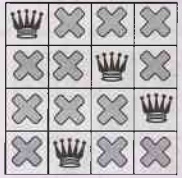
• The solver starts by arbitrarily placing a queen in the upper left corner. That's a hypothesis of sorts; perhaps it will turn out that no solution exists with a queen in the upper left corner.

• Given this hypothesis, what constraints can we propagate? One constraint is that there can be only one queen in a column (the gray Xs below), and another constraint prohibits two queens on the same diagonal (the red Xs below).

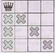
• Our third constraint prohibits queens on the same row:

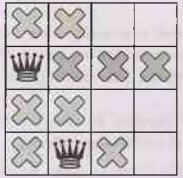
• Our constraints propagated, we can test out another hypothesis, and place a second queen on one of the available remaining squares. Our solver might decide to place in it the first available square in the second column:

• After propagating the diagonal constraint, we can see that it leaves no available squares in either the third column or last row:

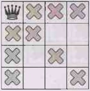
• With no solutions possible at this stage, we need to backtrack. One option is for the solver to choose the other available square in the second column. However, constraint propagation then forces a queen into the second row of the third column, leaving no valid spots for the fourth queen:

• And so the solver must backtrack again, this time all the way back to the placement of the first queen. We have now shown that no solution to the our queens problem will occupy a corner square.

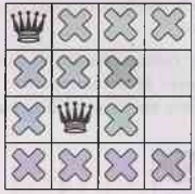
• Since there can be no queen in the corner, the solver moves the first queen down by one, and propagates, leaving only one spot for the second queen:

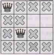
• Propagating again reveals only one spot left for the third queen:

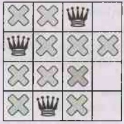
• And for the fourth and final queen:

• This is the first solution! If instructed the solver to stop after finding the first solution, it would end here. Otherwise, it would backtrack again and place the first queen in the third row of the first column.

Scene Labeling

• This is a subproblem of the vision problem, which seeks to deduce facts about the physical world from visual representations of it. In the scene labeling problem we are given a 2-D line drawing of a 3-D scene and must label the components of the drawing in such a way as to make explicit the 3-D structure the drawing represents.

• This problem has been studied extensively since the early 1970s; we will consider a simplified version which was studied by David Waltz as part of his Ph.D. thesis at M.I.T. during this period. The assumptions we make to achieve this simplification are:

1. Every vertex is trihedral (formed by the junction of three planar surfaces; implicitly, we assume that all surfaces are planar).

2. Surfaces do not contain 0-width cracks (lines formed by the junction of coplanar surfaces).

3. No shadows (lines which represent projections of edges onto surfaces along the direction of light sources) are allowed.

4. The scene is viewed from a general viewing position (roughly, for some sufficiently small ε > 0 we can move our viewing point in an arbitrary direction by a distance of ε without any topologically significant change in the resulting 2-D representation).

• It actually turns out, as was revealed by later work on the problem, that assumption 3 is not really a simplification, since the information which can be deduced from the presence and positions of shadows in some sense outweighs the potential for confusion with actual edges they bring with them, but we will follow Waltz' path here and let the assumption stand.

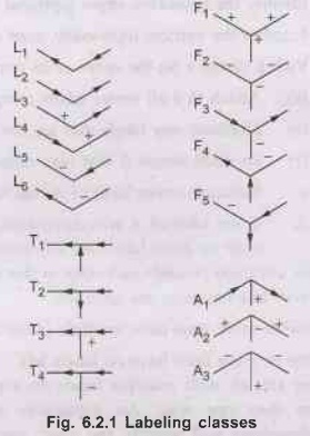
• Although a detailed analysis of the problem is beyond the scope of this lecture, one of the fundamental results of this analysis is that a relatively simple taxonomy of 4 classes of vertices and 4 classes of lines suffices to cover all physical possibilities, modulo the assumptions we have made. While we will not give formal definitions of the classes here, they may be intuitively described as follows:

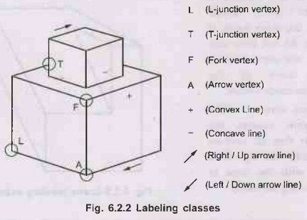
1. L-Junction Vertices: Vertices at which only 2 visible lines meet.

2. T-Junction Vertices: Vertices at which one line segment ends in the middle of another.

3. Fork Vertices: Vertices at which three lines meet, with no angles greater than or equal to 180° between any pair of them.

4. Arrow Vertices: Vertices at which three lines meet, with an angle greater than 180° between one pair of them.

1. Convex Lines: Lines formed by the junction of two visible surfaces for which a line segment connecting the two surfaces would be inside the solids they bound.

2. Concave Lines: Lines formed by the junction of two visible surfaces for which a line segment connecting the two surfaces would be outside the solids they bound.

3. Right / Up Arrow Lines: Lines formed by the junction of one visible and one obscured surface, with the visible surface lying below/to the right of the line.

4. Left / Down Arrow Lines: Lines formed by the junction of one visible and one obscured surface,with the visible surface lying above/to the left of the line.

• Depending on the viewing location, these 4 classes of vertices and 4 classes of lines can be combined to give the eighteen types of vertices shown in the following Fig. 6.2.1.

• Representative examples of each of these classes may be seen in the following drawing:

• As we shall see, the classification of vertices and lines in this way allows us to pose the scene labeling problem as a CSP, with vertices as variables to be labeled with values from the list of classes above; since each class of vertex can only have certain classes of lines meet to form it, the restrictions imposed by the classification of the two vertices at the endpoints of each line must be compatible, 90 which then provides us with the constraints.

• The general algorithm for scene-labeling is as follows:

1. Identify the boundary edges (optional but desirable).

2. Number the vertices (optionally, start with a boundary vertex) in some order.

3. Visit a vertex v (in the order of its numbering) and attempt to label it:

(a) Attach to v all vertex labels compatible with its type.

(b) Eliminate any labels that are not consistent with local constraints.

(c) For each vertex A that was visited in (b),

i. Eliminate every label of A that has no consistent label in v

ii. If any label of A was eliminated, continue propagating the constraints until no more labels are eliminated.

• There are three possible outcomes of this algorithm:

1. Every line has only one label left,

2. One or more lines have multiple labels left, or

3. One or more lines have no labels left.

• If we are left with multiple labels on some lines, the scene can be interpreted in more than one way. An exhaustive search through the remaining possible combinations will identify the valid interpretations. This takes considerably less effort than an exhaustive search the entire search space. On the other hand, if some lines do not have any labels left, the scene violates or more of the assumptions made earlier.

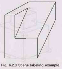
• For instance, vertex J in the above figure violates the assumption that all vertices are trihedral. The algorithm will end with the lines at vertex J having no labels.

Example

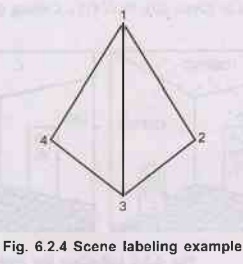
• As an example of the algorithm for scene-labeling, consider the scene shown in the following Fig. 6.2.4.

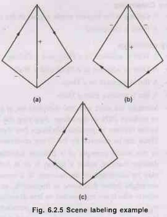
• Vertex 1 is an example of arrow vertices and as such, has three possible labels: (A1, A2, A3). Thus, line (1, 2) has three possible labels : (+, -, ). These constrain the number of possible interpretations that vertex 2 (an L-vertex) can have. Specifically, vertex 2 can have only the following four labels (L1, L4, L5, L6). Call this constraint (i). Vertex 3 can also have three possible labels (A1, A2, A3}. These allow line (2, 3) to have the the following labels: (+, -,. These act as an additional constraint on vertex 2 and together with comstraint (i), enable us to eliminate L4 as viable option. Propagating this back to vertex 1, we can then eliminate A2 as one of the labels on vertex 1. This process can be repeated till all possible constraints have been satisfied. We will be left with three interpretations of the scene.

• These are shown in the following Fig. 6.2.5.

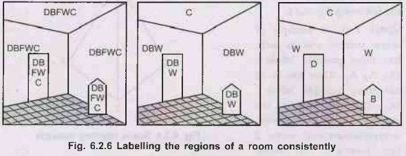
• Fig. 6.2.6, below, illustrates schematically a room interior (from Ballard & Brown, 1982). The set of objects are denoted by regional boundaries and the set of possible labels is {Door (D), Wall (W), Ceiling (C), Floor (F), Bin

• A set of informal constraints might be,

Unary Constraints

• A Ceiling is the highest single region in the image

• A Floor is chequered

N-ary constraints

• A Wall is adjacent to a Floor and a Ceiling.

• A Door is adjacent to a Floor and a Wall.

• A Bin is adjacent to a Floor.

• A Bin is smaller than a Door.

• Inititially we start with the complete set of possible labels for all the regions (2D), or surfaces (3D), in the image. Applying the unary constraints leads to a reduction in the number of possible labellings, but there is still ambiguity in at least 4 cases. These can be resolved by the N-ary constraints.

• In the above example of a discrete labelling regions can only be labelled in a definite manner, either a region is or is not a door. Scene labellings as a whole may be consistent or inconsistent. If a scene cannot be consistently labelled then we might define that scene as impossible, as for example in the case of impossible objects which are represented as line drawings in the AI textbooks. That is all very well, but in an imperfect world it is somewhat unrealistic to ask for certainty in a labelled scene. This leads to the idea of a probabilistic labelling, in which scene elements may be labelled with probability in a continuum (0.0 to 1.0); for example the set of probabilities for a given region in Fig. 6.2.6, might be { Door= 0.1, Bin= 0.3, Floor = 0.1, Wall = 0.2, Ceiling = 0.3}. An algorithm for labelling the scene consistently should update these probabilities to obtain an optimum global labelling satisfying as far as possible the unary characteristics of the regions, and the N-ary characteristics of their relationships. We shall consider this further with the specific examples.xs of subsequent sections.

• Before considering a number of approaches to object recognition by scene labelling, we introduce a few basic definitions. In general, the set of object models is defined,

U = (O₁, O₂, ..., O_n}               ….(6.2.1)

• Each of the n object models may be represented by a set of m(i) primitives, where the parameter, i, denotes the model number (1<<j<=n). These primitives might be surfaces within a B-Rep model, space curves within a wire frame or B-Rep model, volumetric components in a CSG structure and so on.

O_i ={f1, f2,…., f_m(i) }              …..(6.2.2)

• Similarly, the segmented scene consists of a set of m(s) primitives, arising from segmentation of 3D range data or 2D intensity data for example, such that

O_s = {g₁, g₂, …., g_m(s)}              …..(6.2.3)

• The problem is to find the optimum injection mapping, Mp:Os →O;, from the set of scene features defined by equation (6.2.3) to the set of model features define by equation (6.2.2) so that the defined metric for the mapping Mp is a maximum,

M_P  ≥ M_q for all g                  …..(6.2.4)