Introduction of Probabilistic Reasoning

Introduction of Probabilistic Reasoning

AU Dec.-13, May-14,15,18

A agent working in real world environment almost never has access to whole truth about its environment. Therefore, agent needs to work under uncertainity.

Earlier agents we have seen make the epistemological commitment that either the facts (expressed as prepositions) are true, false or else they are unknown. When an agent knows enough facts about its environment, the logical approach enables it to derive plans, which are guaranteed to work.

But when agent works with uncertain knowledge then it might be impossible to construct a complete and correct description of how its actions will work. If a logical agent can not conclude that any perticular course of action achieves its goal, then it will be unable to act.

The right thing logical agent can do is, take a rational decision. The rational decision depends on following things:

• The relative importance of various goals.

• The likelihood and the degree to which, goals will be achieved.

Acting Under Uncertainty

An agent would possess some early basic knowledge of the world (Assume that knowledge is represented in first order logic sentence). Using first order logic to handle real word problem domains fails for three main reasons as discussed below:

1) Laziness:

It is too much work to list the complete set of antecedents or consequents needed to ensure an exceptionless rule and too hard to use such rules.

2) Theoretical ignorance:

A perticular problem may not have complete theory for the domain.

3) Practical ignorance:

Even if all the rules are known, perticular aspects of problem are not checked yet or some details are not considered at all (missing out the details).

The agent's knowledge can provide it with a degree of belief with relevent sentences. To this degree of belief probability theory is applied. Probability assigns a numerical degree of belief between 0 and 1 to each sentence.

Probability provides a way of summarizing the uncertainity that comes from our laziness and ignorance.

Assigning probability of 0 to a given sentence corresponds to an unequivocal belief saying that sentence is false. Assigning probability of 1 corresponds to an unequivocal belief saying that the sentence is true. Probabilities between 0 and 1 correspond to intermediate degree of belief in the truth of the sentence.

The beliefs completely depends on percepts of agent at perticular time. These percepts constitute the evidence on which probability assertions are based. Assignment of probability to a proposition is analogous to saying that whether the given logical sentence (or its negation) is entailed by the knowledge base rather than whether it is true or not. When more sentences are added to knowledge base the entailment keeps on changing. Similarly the probability would also keep on changing with additional knowledge.

All probability statements must therefore, indicate the evidence with respect to which the probability is being assessed. As the agent receives new percepts, its probability assessments are updated to reflect the new evidence. Before the evidence is obtained, we talk about prior or unconditional probability; after the evidence is obtained, we talk about posterior or conditional probability. In most cases, an agent will have some evidence from its percepts and will be interested in computing the posterior probabilities of the outcomes it cares about.

Uncertainty and rational decisions:

The presence of uncertainty drastically changes the way an agent makes decision. At perticular time an agent can have various available decisions, from which it has to make a choice. To make such choices an agent must have a preferences between the different possible outcomes, of the various plans.

A perticular outcome is completely specified state, along with the expected factors related with the outcome.

For example: Consider a car driving agent who wants to reach at airport by a specific time say at 7.30 pm.

Here factors like, whether agent arrived at airport on time, what is the length of waiting duration at the airport are attached with the outcome.

Utility Theory

Utility theory is used to represent and reason with preferences. The term utility in current context is used as "quality of being useful".

Utility theory says that every state has a degree of usefulness called as utility. The agent will prefer the states with higher utility.

The utility of the state is relative to the agent for which utility function is calculated on the basis of agent's preferences.

For example: The pay off functions for games are utility functions. The utility of a state in which black has won a game of chess is obviously high for the agent playing black and low for the agent playing white.

There is no measure that can count test or preferences. Someone loves deep chocolate icecream and someone loves chocochip icecream. A utility function can account for altruistic behavior, simply by including the welfare of other as one of the factors contributing to the agent's own utility.

Decision theory

Preferences as expressed by utilities are combined with probabilities for making rational decisions. This theory, of rational decision making is called as decision theory.

Decision theory can be summarized as,

Decision theory = Probability theory + Utility theory.

• The principle of Maximum Expected Utility (MEU):

Decision theory says that the agent is rational if and only if it chooses the action that yields highest expected utility,averaged over all the possible outcomes of the action.

• Design for a decision theoretic agent:

Following algorithm sketches the structure of an agent that uses decision theory to select actions.

The algorithm

Function: DT-AGENT (percept) returns an action.

Static: belief-state, probabilistic beliefs about the current state of the world. action, the agent's action.

        - Update belief-state based on action and percept

        - Calculate outcome probabilities for actions, given actions descriptions and current belief-state

        - Select action with highest expected utility given probabilities of outcomes and utility information

        - Return action.

A decision therotic agent that selects rational actions.

The decision theoretic agent is identical, at an abstract level, to the logical agent. The primary difference is that the decision theoretic agent's knowledge of the current state is uncertain; the agent's belief state is a representation of the probabilities of all possible actual states of the world.

As time passes, the agent accumulates more evidence and its belief state changes. Given the belief state, the agent can make probabilistic predictions of action outcomes and hence select the action with highest expected utility.

The Basic Probability Notation

The probability theory uses propositional logic language with additional expressivness.

The probability theory uses represent prior probability statements, which apply before any evidence is obtained. The probability theory uses conditional probability statements which include the evidence explicitly.

1. Propositions

1) The propositions (assertions) are attached with the degree of belief.

2) Complex proposition can be formed using standard logical connectives.

For example: [(Cavity = True) (Toothache = False)] and [(Cavity Toothache)] both are same assertions.

• The random variable:

1) The basic element of language is random variable.

2) It reffers to a "part" of the world whose "status" is initially unknown.

For example: In toothache problem 'cavity' is a random variable which can refer to my left wisdom tooth or right wisdom tooth.

3) Random variables are like symbols in propositional logic.

4) Random variables are represented using capital letters. Whereas unknown random variable can be represented with lowercase letter.

For example: P (a) = 1 - P (-a)

5) Each random variable has a domain of values that it can take on. That is domain is, set of allowable values for random variable.

For example: The domain of cavity can be < true, false >

6) A random variable's proposition will assert that what value is drawn for the random variable from its domain.

For example: Cavity = True is proposition.

Saying that "there is" cavity in my lower left wisdom tooth".

7) Random variables are divided into three kinds, depending on their domain. The types are as follows.

i) Boolean random variables: These are random variables that can take up only boolean values.

For example: Cavity, it takes value either true or false.

ii) Discrete random variables: They take values from countable domain. They also include boolean domain. The values in the domain must be mutually exclusive and exhaustive (finite).

For example: Weather, it has domain < sunny, rainy, cloudy, cold >

iii) Continuous random variables: They take values from real numbers. The domain can be either entire real line or subset of it like intervals [2, 3].

For example: X = 4.14 asserts that X has exact value 4.14

Propositions having continuous random variable can have inequalities like X ≤ 4.14.

2. Atomic Events

1) An atomic event is a complete specification of the state of the world about which agent is uncertain.

2) They are represented as variables. These variables are assigned values from the real world.

For example: If the world is consists of cavity and Toothache then there are four distinct atomic events,

a) Cavity = False Ʌ Toothache = True

b) Cavity = False Ʌ Toothache = False

c) Cavity = True Ʌ Toothache = False

d) Cavity = True Ʌ Toothache = True

e) Properties of atomic events

i) They are mutually exclusive - That is at most one can actually be the case. For example: (Cavity Ʌ Toothache) and (Cavity Ʌ ⌐ Toothache) can not both be the case.

ii) The set of all possible atomic events is exhaustive out of which at least one must be the case. That is, the disjunction of all atomic events is logically equivalent to true.

iii) Any particular atomic event entails the truth or falsehood of every proposition, whether simple or complex.

For example -

The atomic event

(Cavity Ʌ⌐ Toothache) entails the truth of cavity and the Falsehood of (cavity → toothache).

iv) Any proposition is logically equivalent to the disjunction of all atomic events that entail the truth of the proposition.

For example: The proposition cavity is equivalent to disjunction of the atomic events (cavityɅtoothache) and (cavity Ʌ ⌐ toothache).

3. Prior Probability (Unconditional Probability)

1) The prior (unconditional) probability is associated with a proposition 'a'.

2) It is the degree of belief accorded to a proposition in the absence of information.

3) It is written as P(a).

For example: The probability that, Ram has cavity = 0.1, then prior probability is written as, P (Cavity = true) = 0.1 or P (Cavity) = 0.1

4) It should be noted that as soon as new information is received, one should reason with the conditional probability of 'a' depending upon new information. 5) When it is required to express probabilities of all the possible values of a random variable, then a vector of values is used. It is represented using P(a). This represents values for the probabilities of each individual state of the 'a'.

For example: P (Weather) = < 0.7, 0.2, 0.08, 0.02 > is representing four equations

P (Weather = Sunny) = 0.7

P (Weather = Rain) = 0.2

P (Weather = Cloudy) = 0.08

P (Weather = Cold) = 0.02

6) The expression P(a) is said to be defining prior probability distribution for the random variable 'a'.

7) To denote probabilities of all random variables combinations, the expression P(a₁, a₂) can be used. This is called as joint probability distribution for random variables a₁, a₂. Any number of random variables can be mentioned in the expression.

8) A simple example of joint probability distribution is,

→ P<Weather, Cavity> can be represented as, 4×2 table of probabilities.

(Weather's probability) (Cavity probability)

9) A joint probability distribution that covers the complete set of random variables is called as full joint probability distribution.

10) A simple example of full joint probability distribution is,

If problem world consists of 3 random variables, wheather, cavity, toothache then full joint probability distribution would be,

P<Weather, Cavity, Toothache>

It will be represented as, 4×2×2, table of probabilities.

11) Prior probability for continuous random variable:

i) For continuous random variable it is not feasible to represent vector of all possible values because the values are infinite. For continuous random variable the probability is defined as a function with parameter x, which indicates that random variable takes some value x.

For example: Let random variable x denotes the tomorrow's temperature in Chennai. It would be represented as,

P(X = x) = U [25 – 37] (x).

This sentence express the belief that X is distributed uniformly between 25 and 37 degrees celcius.

ii) The probability distribution for continuous random variable has probability density function.

4. Conditional Probability

1) When agent obtains evidence concerning previously unknown random variables in the domain, then prior probability are not used. Based on new information conditional or posterior probabilities are calculated.

2) The notation is P(a | b) where a and b are any proposition.

The 'P' is read as "the probability of a given that all we know is b". That is when b is known it indicates probability of a.

For example: P (Cavity | Toothache) = 0.8

it means that, if patient has toothache (and no other information is known) then the chances of having cavity are = 0.8

3) Prior probability are infact special case of conditional probability. It can be represented as P(a) which means that probability 'a' is conditioned on no evidence.

4) Conditional probability can be defined interms of unconditional probabilities. The equation would look like,

P(a/b) =P(aɅb) / P(b), it holds whenever P(b) > 0                     …(7.1.1)

The above equation can also be written as,

P(a Ʌ b) = P(a | b) P(b)

This is called as product rule. In other words it says, for 'a' and 'b' to be true we need 'b' to be true and we need a to be true given b. It can be also written as,

P(a Ʌ b)= P(b | a) P(a).

5) Conditional probability are used for probabilistic inferencing.

6) P notation can be used for conditional distribution. P(x | y) gives the values of P(X = x_i | Y = y_j) for each possible i, j. following are the individual equations,

P(X = x₁ ^ Y = y₁) = P(X = x₁ |Y = y₁) P(Y = y₁)

P(X = x₁ ^ Y = y₂) = P(X = x₁ |Y = y₂) P(Y = y₂)

These can be combined into a single equation as,

P(X, Y) = P(X | Y) P(Y)

7) Conditional probabilities should not be treated as logical implications. That is, "When 'b' holds then probability of 'a' is something", is a conditional probability o and not to be mistake as logical implication. It is wrong on two points, one is, P(a) always denotes prior probability. For this it do not require any evidence. P(a | b) = 0.7, is immediately relevant when b is available evidence. This will keep on altering. When information is updated logical Implications do not change over time.

5. The Probability Axioms

Axioms gives semantic of probability statements. The basic axioms (Kolmogorov's axioms) serve to define the probability scale and its end points.

1) All probabilities are between 0 and 1. For any proposition a, 0 ≤ P(a) ≤1.

2) Necessarily true (i.e, valid) propositions have probability 1, and necessarily false (i.e., unsatisfiable) propositions have probability 0.

P(true) = 1    P(false) = 0

3) The probability of a disjunction is given by

P (a v b) = P(a) + P(b) - P(a Ʌ b)

This axiom connects the probabilities of logically related propositions. This rule states that, the cases where 'a' holds, together with the cases where 'b' holds, certainly cover all the causes where 'a v b' holds; but summing the two sets of cases counts their intersection twice, so we need to subtract P(a Ʌ b).

Note The axioms deal only with prior probabilities rather than conditional probabilities; this is because prior probability can be defined in terms of conditional probability.

Using the axioms of probability:

From basic probability axioms following facts can be deduced.

 P(a v¬ a) = P(a) + P(¬a) - P(a Ʌ¬a) (by axiom 3 with b = ¬ a)

P(true) = P(a) + P(¬ a) - P(false) (by logical equivalence)

1 = P(a) + P(¬ a) (by axiom 2)

P(¬ a) = 1 - P(a) (by algebra).

• Let the discrete variable D have the domain <d₁,....., d_n>.

Then, Σⁿ_i=1 P(D=d_i) = 1.

That is, any probability distribution on a single variable must sum to 1.

• It is also true that any joint probability distribution on any set of variables must sum to 1. This can be seen simply by creating a single megavariable whose domain is the cross product of the domains of the original variables.

• Atomic events are mutually exclusive, so the probability of any conjunction of atomic events is zero, by axiom 2.

• From axiom 3, we can derive the following simple relationship: The probability of a proposition is equal to the sum of the probabilities of atomic events in which it holds; that is P(a) = Σ_{ei ε e(a)} P(e_i)        …..(7.1.2)

6. Inference using Full Joint Distribution

Probabilistic inference means, computation from observed evidence of posterior probabilities, for query propositions. The knowledge base used for answering the query is represented as full joint distribution. Consider simple example, consists of three boolean variables, toothache, cavity, catch. The full joint distribution is 2×2×2, as shown below.

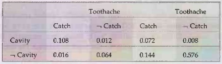
Note that the probability in the joint distribution sum to 9.

• One particular common task in inferencing is to extract the distribution over some subset of variables or a single variable. This distribution over some variables or single variables is called as marginal probability.

For example: P(Cavity) = 0.108 +0.012+ 0.072 + 0.008. = 0.2

This process is called as marginalization or summing. Because the variables other than 'cavity' (that is whose probability is being counted) are summed out.

• The general marginalization rule is as follows,

For any sets of variables Y and Z,

P(Y) = Σ _z P(Y, z).                              ….(7.1.3)

It indicates that distribution Y can be obtained by summing out all the other paulay to variables from any joint distribution X containing Y.

• Variant of above example of general marginalization rule involved the conditional to to probabilities using product rule.

P(Y) = Σ _z P(Y | z) P(z)              ….(7.1.4)

This rule is conditioning rule.

For example: Computing probability of a cavity, given evidence of a toothacheis as follows:

P(Cavity | Toothache) =P(Cavity Ʌ Toothache) /P(Toothache) = 0.108+0.012 / 0.108+0.012+0.016+0.064 = 0.6

• Normalization constant: It is variable that remains constant for the distribution, which ensures that it adds in to 1. a is used to denote such constant.

For example: We can compute the probability of a cavity, given evidence of a toothache, as follows:

P(Cavity | Toothache) = P(Cavity Ʌ Toothache)/ P(Toothache) = 0.108+0.012/

0.108+0.012+0.016+0.064 = 0.6

Just to check we can also compute the probability that there is no cavity given a toothache:

P( Cavity / Toothache)= P (¬Cavity Ʌ Tootache) /P (Toothache) = 0.016+ 0.064 / 0.108+0.012+ 0.016+ 0.064 = 0.4

Notice that in these two calculations the term 1/P (toothache) remains constant, no matter which value of cavity we calculate. With this notation we can write above two equations in one.

P(Cavity | Toothache) = αP(Cavity, Toothache)

= α [P(Cavity, Toothache, Catch) + P(Cavity, Toothache,  ¬ Catch)]

= α [< 0.108, 0.016> + <0.012, 0.064>]

= α <0.12, 0.08> = <0.6, 0.4>

From above one can extract a general inference procedure.

Consider the case in which query involves a single variable. The notation used is let X be the query variable (cavity in the example), let E be the set of evidence variables (just toothache in the example) let e be the observed values for them, and let Y be the remaining unobserved variable (just catch in the example). The query is P(X/e) and can be evaluated as

P(X | e) = α P(X, e) = α Σ _y P(X, e, y)                 ……(7.1.5)

where the summation is over all possible ys (i.e. all possible combinations of values of the unobserved variables 'y'). Notice that together the variables, X, E and Y constitute the complete set of variables for the domain, so P (X, e, y) is simply a subset of probabilities from the full joint distribution.

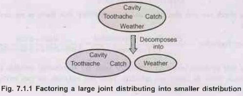
7. Independance

It is a relationship between two different sets of full joint distributions. It is also called as marginal or absolute independance of the variables. Independence indicates that whether the two full joint distributions affects probability of each other.

The independance between variables X and Y can be written as follows,

P(X | Y) = P(X) or P(Y | X) = P(Y) or P(X, Y) = P(X) P(Y)

• For example: The weather is independant of once dental problem. Which can be shown as below equation.

P(Toothache, Catch, Cavity, Weather) = P(Toothache, Catch, Cavity) P(Weather).

• Following diagram shows factoring a large joint distributing into smaller distributions, using absolute independence. Weather and dental problems are independent.

8. Bayes' Rule

Bayes' rule is derived from the product rule.

The product rule can be written as,

P(a Ʌ b)=P(a | b) P(b)           .…(7.1.6)

P(a Ʌ b)=P(b | a) P(a)                .... (7.1.7)

[because conjunction is commutative]

Equating right sides of equation (7.1.6) and equation (7.1.7) and dividing by P(a),

P(b | a) = P(a | b)P(b) / P(a)

This equation is called as Bayes' rule or Bayes' theorem or Bayes' law. This rule is very useful in probabilistic inferences.

Generalized Bayes' rule is,

P(Y | X) = P(X | Y) P(Y) / P(X)

(where P has same meanings)

We can have more general version, conditionalized on some background evidence e.

P(Y | X, e) = P(X |Y, e) P(Y | e) / P(X | e)

General form of Bays' rule with normalization's

P(y | x) = α P(x | y) P(y).

Applying Bays' Rule:

1) It requires total three terms (1 conditional probability and 2 unconditional Probabilities). For computing one conditional probability.

For example: Probability of patient having low sugar has high blood pressure is

50 %.

Let, M be proposition, 'patient has low sugar'.

S be a proposition, 'patient has high blood pressure'.

Suppose we assume that, doctor knows following unconditional fact,

i) Prior probabilition of (m) = 1/50,000.

ii) Prior probability of (s) = 1/20.

Then we have,

P(s | m) = 0.5

P(m) = 1 | 50000

P(s) = 1 | 20

P(m/s) = P(s | m) P(m) / P(s)

= 0.5×1/50000 /1/20

= 0.0002

That is, we can expect that 1 in 5000 with high B.P. will has low sugar.

2) Combining evidence in Bayes' rule.

Bayes rule is helpful for answering queries conditioned on evidences.

For example: Toothache and catch both evidences are available then cavity is sure to exist. Which can be represented as,

P(Cavity | Toothache ^ Catch) = α <0.108, 0.016> ≈ <0.871, 0.129>

By using Bayes' rule to reformulate the problem:

P(Cavity | Toothache ^ Catch) = α P(Toothache A Catch | Cavity) P(Cavity)    ……(7.1.8)

For this reformulation to work, we need to know the conditional probabilities of the conjunction Toothache Catch for each value of Cavity. That might be feasible for just two evidence variables, but again it will not scale up.

If there are n possible evidence variable (X-rays, diet, oral hygiene, etc.), then there are 2ⁿ possible combinations of observed values for which we would need to know conditional probabilities.

The notion of independence can be used here. These variables are independent, however, given the presence or the absence of a cavity. Each is directly caused by the cavity, but neither has a direct effect on the other. Toothache depends on the state of the nerves in the tooth, where as the probe's accuracy depends on the dentist's skill, to which the toothache is irrelevant.

Mathematically, this property is written as,

P(Toothache ^ Catch | Cavity) = P(Toothache | Cavity) P(Catch | Cavity) .…(7.1.9)

This equation expresses the conditional independence of toothache and catch, given cavity.

Substitute equation (7.1.3) into (7.1.4) to obtain the probability of a cavity:

P (Cavity | Toothache ^Catch) = α P (Toothache | Cavity) P (Catch | Cavity) P (Cavity)

Now, the information requirement are the same as for inference using each piece of evidence separately the prior probability P(Cavity) for the query variable and the conditional probability of each effect, given its cause.

Conditional independence assertions can allow probabilistic systems to scale up; more over, they are much more commonly available than absolute independence assertions. When their are 'n' variables given that they are all conditionally independent, the size of the representation grows as O(n) instead of O(2n).

For example -

Consider dentistry example, in which a single cause, directly influences a number of effects, all of which are conditionally independent, given the cause.

The full joint distribution can be written as,

P(Cause, Effect₁,..., Effect_n) = P(Cause) II P(Effect_i | Cause).

Such a probability distribution is called as naive Bayes' model - "naive" because it is often used (as a simplifying assumption) in cases where the "effect" variables are not conditionally independent given the cause variable. The naive Bayes model is sometimes called as Bayesian classifier.