Describing Data with Tables

Describing Data with Tables

Frequency Distributions for Quantitative Data

• Frequency distribution is a representation, either in a graphical or tabular format, that displays the number of observations within a given interval. The interval size depends on the data being analyzed and the goals of the analyst.

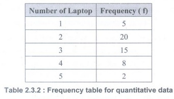
• In order to find the frequency distribution of quantitative data, we can use the following table that gives information about "the number of smartphones owned per family."

• For such quantitative data, it is quite straightforward to make a frequency distribution table. People either own 1, 2, 3, 4 or 5 laptops. Then, all we need to do is to find the frequency of 1, 2, 3, 4 and 5. Arrange this information in table format and called as frequency table for quantitative data.

• When observations are sorted into classes of single values, the result is referred to as a frequency distribution for ungrouped data. It is the representation of ungrouped data and is typically used when we have a smaller data set.

• A frequency distribution is a means to organize a large amount of data. It takes data from a population based on certain characteristics and organizes the data in a way that is comprehensible to an individual that wants to make assumptions about a given population.

• Types of frequency distribution are grouped frequency distribution, ungrouped frequency distribution, cumulative frequency distribution, relative frequency distribution and relative cumulative frequency distribution

1. Grouped data:

• Grouped data refers to the data which is bundled together in different classes or categories.

• Data are grouped when the variable stretches over a wide range and there are a large number of observations and it is not possible to arrange the data in any order, as it consumes a lot of time. Hence, it is pertinent to convert frequency into a class group called a class interval.

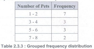
• Suppose we conduct a survey in which we ask 15 familys how many pets they have in their home. The results are as follows:

1, 1, 1, 1, 2, 2, 2, 3, 3, 4, 5, 5, 6, 7, 8

• Often we use grouped frequency distributions, in which we create groups of values and then summarize how many observations from a dataset fall into those groups. Here's an example of a grouped frequency distribution for our survey data :

Guidelines for Constructing FD

1. All classes should be of the same width.

2. Classes should be set up so that they do not overlap and so that each piece of data belongs to exactly one class.

3. List all classes, even those with zero frequencies.

4. There should be between 5 and 20 classes.

5. The classes are continuous.

• The real limits are located at the midpoint of the gap between adjacent tabled boundaries; that is, one-half of one unit of measurement below the lower tabled boundary and one-half of one unit of measurement above the upper tabled boundary.

• Table 2.3.4 gives a frequency distribution of the IQ test scores for 75 adults.

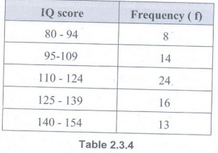
• IQ score is a quantitative variable and according to Table, eight of the individuals have an IQ score between 80 and 94, fourteen have scores between 95 and 109, twenty-four have scores between 110 and 124, sixteen have scores between 125 and 139 and thirteen have scores between 140 and 154.

• The frequency distribution given in Table is composed of five classes. The classes are: 80-94, 95-109, 110- 124, 125-139 and 140- 154. Each class has a lower class limit and an upper class limit. The lower class limits for this distribution are 80, 95, 110, 125 and 140. The upper class limits are 94,109, 124, 139 and 154.

• If the lower class limit for the second class, 95, is added to the upper class limit for the first class,94 and the sum divided by 2, the upper boundary for the first class and the lower boundary for the second class is determined. Table 2.3.5 gives all the boundaries for Table 2.3.5.

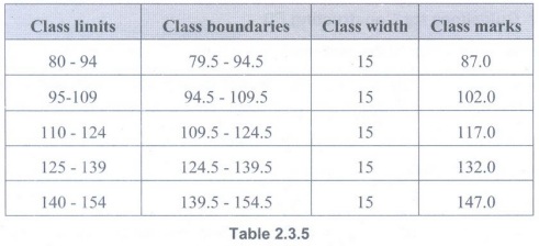
• If the lower class limit is added to the upper class limit for any class and the sum divided by 2, the class mark for that class is obtained. The class mark for a class is the midpoint of the class and is sometimes called the class midpoint rather than the class mark.

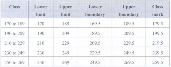
Example 2.3.1: Following table gives the frequency distribution for the cholesterol values of 45 patients in a cardiac rehabilitation study. Give the lower and upper class limits and boundaries as well as the class marks for each class.

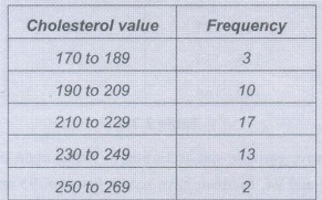
• Solution: Below table gives the limits, boundaries and marks for the classes.

Example 2.3.2: The IQ scores for a group of 35 school dropouts are as follows:

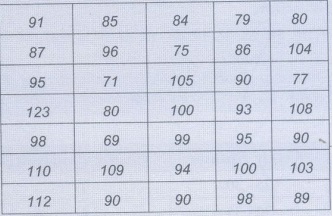
a) Construct a frequency distribution for grouped data.

b) Specify the real limits for the lowest class interval in this frequency distribution.

• Solution: Calculating the class width

(123-69)/ 10=54/10=5.4≈ 5

a) Frequency distribution for grouped data

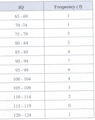
b) Real limits for the lowest class interval in this frequency distribution = 64.5-69.5.

Example 2.3.3: Given below are the weekly pocket expenses (in Rupees) of a group of 25 students selected at random.

37, 41, 39, 34, 41, 26, 46, 31, 48, 32, 44, 39, 35, 39, 37, 49, 27, 37, 33, 38, 49, 45, 44, 37, 36

Construct a grouped frequency distribution table with class intervals of equal widths, starting from 25-30, 30-35 and so on. Also, find the range of weekly pocket expenses.

Solution:

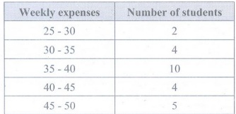
• In the given data, the smallest value is 26 and the largest value is 49. So, the range of the weekly pocket expenses = 49-26=23.

Outliers

• 'In statistics, an Outlier is an observation point that is distant from other observations.'

• An outlier is a value that escapes normality and can cause anomalies in the results obtained through algorithms and analytical systems. There, they always need some degrees of attention.

• Understanding the outliers is critical in analyzing data for at least two aspects:

a) The outliers may negatively bias the entire result of an analysis;

b) The behavior of outliers may be precisely what is being sought.

• The simplest way to find outliers in data is to look directly at the data table, the dataset, as data scientists call it. The case of the following table clearly exemplifies a typing error, that is, input of the data.

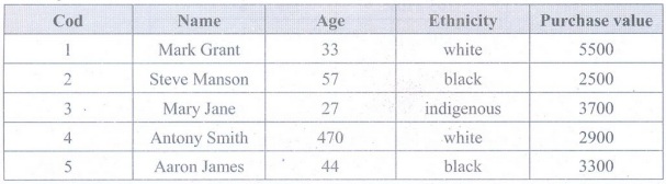
• The field of the individual's age Antony Smith certainly does not represent the age of 470 years. Looking at the table it is possible to identify the outlier, but it is difficult to say which would be the correct age. There are several possibilities that can refer to the right age, such as: 47, 70 or even 40 years.

Relative and Cumulative Frequency Distribution

• Relative frequency distributions show the frequency of each class as a part or fraction of the total frequency for the entire distribution. Frequency distributions can show either the actual number of observations falling in each range or the percentage of observations. In the latter instance, the distribution is called a relative frequency distribution.

• To convert a frequency distribution into a relative frequency distribution, divide the frequency for each class by the total frequency for the entire distribution.

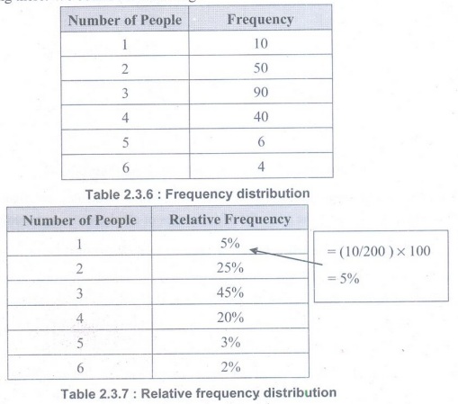
• A relative frequency distribution lists the data values along with the percent of all observations belonging to each group. These relative frequencies are calculated by dividing the frequencies for each group by the total number of observations.

• Example: Suppose we take a sample of 200 India family's and record the number of people living there. We obtain the following:

Cumulative frequency:

• A cumulative frequency distribution can be useful for ordered data (e.g. data arranged in intervals, measurement data, etc.). Instead of reporting frequencies, the recorded values are the sum of all frequencies for values less than and including the current value.

• Example: Suppose we take a sample of 200 India family's and record the number of people living there. We obtain the following:

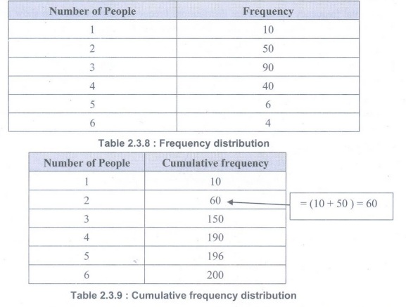
• To convert a frequency distribution into a cumulative frequency distribution, add to the frequency of each class the sum of the frequencies of all classes ranked below it.

Frequency Distributions for Qualitative (Nominal) Data

• In the set of observations, any single observation is a word, numerical code or letter, then data are qualitative data. Frequency distributions for qualitative data are easy to construct.

• It is possible to convert frequency distributions for qualitative variables into relative frequency distribution.

• If measurement is ordinal because observations can be ordered from least to most, cumulative frequencies can be used.