Contiguous Memory Allocation with Variable Size Partitions

Contiguous Memory Allocation with Variable Size Partitions

AU: Dec.-17

• The use of unequal size partitions provides a degree of flexibility to fixed partitioning. In dynamic partitioning, the partitions are of variable length and number.

• In noncontiguous memory allocation, a program is divided into blocks that the system may place in nonadjacent slots in main memory.

• This allocation method do not suffer from internal fragmentation, because a process partition is exactly the size of the process.

• Fig. 4.4.1 shows noncontiguous memory allocation method. Operating system maintain the table which contains the memory areas allocated to process and free memory. Memory management unit use this information for allocating processes.

• Table contains information about memory starting address for process/program and their size.

• CPU sends the logical address of the process to the MMU and the MMU uses the memory allocation information stored in the table for calculating logical address. We called this address as effective memory address of the data/instruction.

Difference between Contiguous and Noncontiguous Memory

Fragmentation

• Fragmentation are of two types:

1. Internal fragmentation.

2. External fragmentation.

• In fragmentation, OS cannot use certain area of available memory.

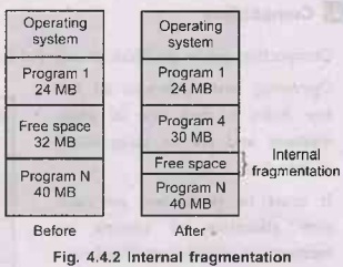
Internal fragmentation

• There is wasted space internal to a partition due to the fact that the block of data loaded is smaller than the partition is called as internal fragmentation.

• Fig. 4.4.2 shows an internal fragmentation.

• To keep track of this free hole is overhead for system.

External fragmentation

• It occurs when enough total main memory space exists to satisfy a request, but it is not contiguous, storage fragmentated into a large number of small holes.

• Fig. 4.4.3 shows external fragmentation.

• Following are the solution for external fragmentation:

1. Compaction

2. Logical address space of a process/program

Difference between Internal and External Fragmentation

Compaction

• Compaction solves problem of external fragmentation. Fig. 4.4.4 shows compaction.

• Operating system moves all the free holes to one side of main memory and creates large block

• It must be performed on each new allocation of process to memory or completion of process for memory. System must also maintain relocation information.

• All free blocks are brought together as one large block of free space. Compaction requires dynamic relocation.

• Compaction has a cost and selection of an optimal compaction strategy is difficult. One method for compaction is swapping out those processes that are to be moved within the memory and swapping them into different memory locations.

• Compaction is not always possible. Compaction is time consuming method and wastage of the CPU time.

Garbage collection

• Some programs use dynamic data structures. These programs dynamically use and discard memory space. Technically, the deleted data items release memory locations.

• But, in practice the OS does not collect such free space immediately for allocation. This is because that affects performance. Such areas, therefore are called garbage.

• When such garbage exceeds a certain threshold the OS would not have enough memory available for any further allocation.

Placement Algorithms

• In an environment that supports dynamic memory allocation, the memory manager must keep a record of the usage of each allocatable block of memory. This record could be kept by using almost any data structure that implements linked lists.

• An obvious implementation is to define a free list of block descriptors, with each descriptor containing a pointer to the next descriptor, a pointer to the block and the length of the block.

• The memory manager keeps a free list pointer and inserts entries into the list in some order conductive to its allocation strategy. A number of strategies are used. to allocate space to the processes that are competing for memory.

• Fig. 4.4.5 shows the placement algorithm.

Best fit: The allocator places a process in the smallest block of unallocated memory in which it will fit. For example, suppose a process requests 12 kB of memory and the memory manager currently has a list of unallocated blocks of 6 kB, 14 kB, 19 kB, 11 kB and 13 kB blocks. The best-fit strategy will allocate 12 kB of the 13 kB block to the process.

• Best fit chooses the block that is closest in the size to the request.

Problems of best fit

• It requires an expensive search of the entire free list to find the best hole.

• More importantly, it leads to the creation of lots of little holes that are not big enough to satisfy any requests. This situation is called fragmentation and is a problem for all memory-management strategies, although it is particularly bad for best-fit.

Solution: One way to avoid making little holes is to give the client a bigger block than it asked for. For example, we might round all requests up to the next larger multiple of 64 bytes. That doesn't make the fragmentation go away, it just hides it. Unusable space in the form of holes is called external fragmentation.

2. Worst fit: The memory manager places a process in the largest block of unallocated memory available. The idea is that this placement will create the largest hold after the allocations, thus increasing the possibility that compared to best fit; another process can use the remaining space. Using the same example as above, worst fit will allocate 12 kB of the 19 kB block to the process, leaving a 7 kB block for future use.

3. First fit: There may be many holes in the memory, so the operating system, to reduce the amount of time it spends analyzing the available spaces, begins at the start of primary memory and allocates memory from the first hole it encounters large enough to satisfy the request. Using the same example as above, first fit will allocate 12 kB of the 14 kB block to the process.

4. Next fit: The first fit approach tends to fragment the blocks near the beginning of the list without considering blocks further down the list. Next fit is a variant of the first-fit strategy. The problem of small holes accumulating is solved with next fit algorithm, which starts each search where the last one left off, wrapping around to the beginning when the end of the list is reached (a form of one-way elevator).

• Notice in the diagram above that the best fit and first fit strategies both leave a tiny segment of memory unallocated just beyond the new process.

Example 4.4.1 Given memory partitions of 100 K, 500 K, 200 K, 300 K and 600 K (in order) how would each of the first-fit, best-fit and worst-fit algorithms place processes of 212 K, 417 K, 112 K and 426 K (in order)? Which algorithm makes the most efficient use of memory?

Solution: First-fit:

212 K is put in 500 K partition

417 K is put in 600 K partition

112 K is put in 288 K partition (new partition 288 K = 500 K - 212 K)

426 K must wait.

Best-fit:

212 K is put in 300 K partition

417 K is put in 500 K partition

112 K is put in 200 K partition

426 K is put in 600 K partition

Worst-fit:

212 K is put in 600 K partition

417 K is put in 500 K partition

112 K is put in 388 K partition (600 K - 212 K)

426 K must wait

In this example, Best-fit turns out to be the best.

University Question