Collision Resolution Techniques

Collision Resolution Techniques

Definition: If collisions occur then it should be handled by applying some techniques, such techniques are called collision handling techniques.

Chaining

1. Chaining without replacement

In collision handling method chaining is a concept which introduces an additional field with data i.e. chain. A separate chain table is maintained for colliding data. When collision occurs we store the second colliding data by linear probing method. The address of this colliding data can be stored with the first colliding element in the chain table, without replacement.

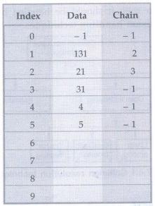
For example consider elements,

131, 3, 4, 21, 61, 6, 71, 8, 9

From the example, you can see that the chain is maintained the number who demands for location 1. First number 131 comes we will place at index 1. Next comes 21 but collision Fig. 7.4.2 Chaining without replacement occurs so by linear probing we will place 21 at index 2, and chain is maintained by writing 2 in chain table at index 1 similarly next comes 61 by linear probing we can place 61 at index 5 and chain will be maintained at index 2. Thus any element which gives hash key as 1 will be stored by linear probing at empty location but a chain is maintained so that traversing the hash table will be efficient.

The drawback of this method is in finding the next empty location. We are least bothered about the fact that when the element which actually belonging to that empty location cannot obtain its location. This means logic of hash function gets disturbed.

2. Chaining with replacement

As previous method has a drawback of loosing the meaning of the hash function, to overcome this drawback the method known as chaining with replacement is introduced. Let us discuss the example to understand the method. Suppose we have to store following elements :

131, 21, 31, 4, 5

Now next element is 2. As hash function will indicate hash key as 2 but already at index 2. We have stored element 21. But we also know that 21 is not of that position at which currently it is placed.

Hence we will replace 21 by 2 and accordingly chain table will be updated. See the table :

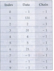
The value -1 in the hash table and chain table indicate the empty location

The advantage of this method is that the meaning of hash function is preserved. But each time some logic is needed to test the element, whether it is at its proper position.

Open Addressing

Open addressing is a collision handling technique in which the entire hash table is searched in systematic way for empty cell to insert new item if collision occurs.

Various techniques used in open addressing are

1. Linear probing     2. Quadratic probing       3. Double hashing

1. Linear probing    

When collision occurs i.e. when two records demand for the same location in the hash table, then the collision can be solved by placing second record linearly down wherever the empty location is found.

For example

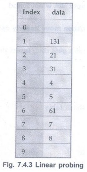
In the hash table given in Fig 7.4.3 the hash function used is number % 10. If the first 131 then 131 % 10= 1 i.e. remainder is 1 so hash key = 1. That means we are supposed to place the record at index 1. Next number is 21 which gives hash key 1 as 21 % 10 1. But already 131 is placed at index 1. That means collision is occurred. We will now apply linear probing. In this method, we will search the place for number 21 from location of 131. In this case we can place 21 at index 2. Then 31 at index 3. Similarly 61 can be stored at 6 because number 4 and 5 are stored before 61. Because of this technique, the searching becomes efficient, as we have to search only limited list to obtain the desired number.

Ex. 7.4.1: Implement the hash table and perform collision handling by Linear probing

Sol. :

#include <stdio.h>

#include <conio.h>

void display(int a[], int n)

{

// Displaying complete hash table

for (int i = 0; i < n; i++)

{

printf("\n %d %d",i,a[i]);

}

}

void Linear_prob(int table[], int tsize,int num)

{

int key = num % tsize; //Computing the hash key using hash function

while (table[key]!= -1) //if empty slot is not found

{

key=(key+1)%tsize; //then move linearly dow in search of empty slot

}

table[key]=num ; //if empty slot gets then insert the element

display(table, tsize);

}

int main()

{

int SIZE = 10;// Size of the hash table

int num;

int hash_table[SIZE];

char ans;

// Initializing the hash table

for (int i=0; i < SIZE; i++)

{

hash_table[i] -1;//-1 indicates empty slot

}

do

{

printf("\nEnter The Number: ");

scanf("%d", &num); //This element is to be inserted in hash table

Linear_prob(hash_table,SIZE,num);

printf("\n Do U Wish To Continue?(y/n)");

 ans = getch();

} while(ans=='y');

return 0;

}

Output

Enter The Number: 131

0 -1

1 131

2 -1

3 -1

4 -1

5 -1

6 -1

7 -1

8 -1

9 -1

Do U Wish To Continue?(y/n)

Enter The Number: 21

0 -1

1 131

2 21

3 -1

4 -1

5 -1

6 -1

7 -1

8 -1

9 -1

Do U Wish To Continue? (y/n)

Enter The Number: 3

0 -1

1 131

2 21

3 3

4 -1

5 -1

6 -1

7 -1

8 -1

9 -1

Do U Wish To Continue? (y/n)

Enter The Number: 4

0 -1

1 131

2 21

3 3

4 4

5 -1

6 -1

7 -1

8 -1

9 -1

Do U Wish To Continue?(y/n)

Enter The Number: 5

0 -1

1 131

2 21

3 3

4 4

5 5

6 -1

7 -1

8 -1

9 -1

Do U Wish To Continue?(y/n)

Enter The Number: 8

0 -1

1 131

2 21

3 3

4 4

5 5

6 -1

7 -1

8 8

9 -1

Do U Wish To Continue?(y/n)

Enter The Number: 9

0 -1

1 131

2 21

3 3

4 4

5 5

6 -1

7 -1

8 8

9 9

Do U Wish To Continue?(y/n)

Enter The Number: 18

0 18

1 131

2 21

3 3

4 4

5 5

6 -1

7 -1

8 8

9 9

Do U Wish To Continue?(y/n)

Enter The Number: 33

0 18

1 131

2 21

3 3

4 4

5 5

6 33

7 -1

8 8

9 9

Do U Wish To Continue? (y/n)

Problem with linear probing

One major problem with linear probing is primary clustering. Primary clustering is a process in which a block of data is formed in the hash table when collision is resolved.

For example:

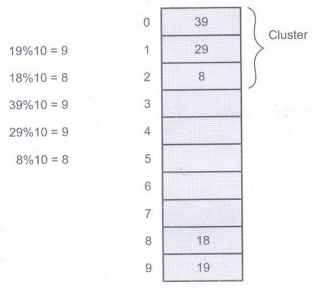
This clustering problem can be solved by quadratic probing.

2. Quadratic probing

Quadratic probing operates by taking the original hash value and adding successive values of an arbitrary quadratic polynomial to the starting value. This method uses following formula -

H_i(key) = (Hash(key)+i²)%m

where m can be a table size or any prime number.

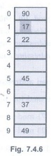
For example: If we have to insert following elements in the hash table with table size 10: 37, 90, 55, 22, 11, 17, 49, 87.

We will fill the hash table step by step

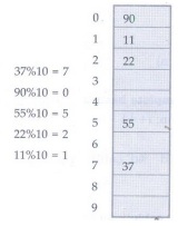
Now if we want to place 17 a collision will occur as 17% 10=7 and bucket 7 has already an element 37. Hence we will apply quadratic probing to insert this record in the hash table.

H_i(key)=(Hash(key)+i²)%m

we will choose value i = 0, 1, 2, whichever is applicable.

Consider i = 0 then

(17+0²) % 10 = 7

(17+1²) % 10 = 8, when i = 1

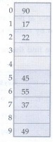
The bucket 8 is empty hence we will place the element at index 8.

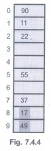
Then comes 49 which will be placed at index 9.

49%10 = 9

Now to place 87 we will use quadratic probing.

(87+0)%10 = 7

(87 + 1)%10 = 8...but already occupied

(87 +22)%10 = 1…already occupied

(87+32)%10 = 6... this slot is free

We place 87 at 6th index.

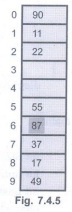
It is observed that if we want to place all the necessary elements in the hash table the size of divisor (m) should be twice as large as total number of elements.

Ex. 7.4.2: Write a C program to implement Quadratic probing.

Sol. :

#include <stdio.h>

#include<conio.h>

void display(int a[], int n)

{

// Displaying complete hash table

for (int i = 0; i < n; i++)

{

printf("\n %d %d",i,a[i]);

}

}

void Quadratic_prob(int table[], int tsize,int num)

{

int key= num % tsize;//computing the hash key using mod function

// Insert in the table if there is empty slot

if (table[key]==-1)

table[key] = num;

else

{

for (int i = 0; i < tsize; i++)//using formula for quadratic probing

{

int index = (key + i* i) % tsize;

if (table[index]==-1)//if empty slot is found

{

table[index] = num;//then insert element at that index

break;

}

}

}

display(table,tsize);

}

int main()

{

int SIZE = 10;//Size of the hash table

int num;

int hash_table[SIZE];

char ans;

// Initializing the hash table

for (int i== 0; i < SIZE; i++)

{

hash_table[i]= -1;//-1 indicates empty slot

}

do

{

printf("\nEnter The Number: ");

scanf("%d", &num);//Number to be inserted in the hash table

Quadratic_prob(hash_table,SIZE,num);

printf("\n Do U Wish To Continue?(y/n)");

ans = getch();

} while(ans =='y');

return 0;

}

Output

Enter The Number: 37

0 -1

1 -1

2 -1

3 -1

4 -1

5 -1

6 -1

7 37

8 -1

9 -1

Do U Wish To Continue?(y/n)

Enter The Number: 90

0 90

1 -1

2 -1

3 -1

4 -1

5 -1

6 -1

7 37

8 -1

9 -1

Do U Wish To Continue?(y/n)

Enter The Number: 55

0 90

1 -1

2 -1

3 -1

4-1

5 55

6 -1

7 37

8 -1

9 -1

Do U Wish To Continue? (y/n)

Enter The Number: 22

0 90

1 -1

2 22

3 -1

4 -1

5 55

6 -1

7 37

8 -1

9 -1

Do U Wish To Continue?(y/n)

Enter The Number: 11

0 90

1 11

2 22

3 -1

4 -1

5 55

6 -1

7 37

8 -1

9 -1

Do U Wish To Continue?(y/n)

Enter The Number: 17

0 90

1 11

2 22

3 -1

4 -1

5 55

6-1

7 37

8 17

9 -1

Do U Wish To Continue? (y/n)

Enter The Number: 49

0 90

1 11

2 22

3 -1

4 -1

5 55

6 -1

7 37

8 17

9 49

Do U Wish To Continue?(y/n)

Enter The Number: 87

0 90

1 11

2 22

3 -1

4 -1

5 55

6 87

7 37

8 17

9 49

Do U Wish To Continue? (y/n)

3. Double hashing

Double hashing is technique in which a second hash function is applied to the key when a collision occurs. By applying the second hash function we will get the number of positions from the point of collision to insert.

There are two important rules to be followed for the second function :

• It must never evaluate to zero.

• Must make sure that all cells can be probed.

The formula to be used for double hashing is

H₁(key) = key mod tablesize

H₂(key) = M - ( key mod M)

where M is a prime number smaller than the size of the table.

Consider the following elements to be placed in the hash table of size 10

37, 90, 45, 22, 17, 49, 55

Initially insert the eleme nts using the formula for H1(key).

Insert 37, 90, 45, 22.

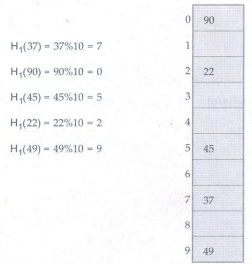
Now if 17 is to be inserted then

H₁(17) = 17% 10 = 7

H₂(key) = M - (key%M)

Here M is a prime number smaller than the size of the table. Prime number smaller than table size 10 is 7.

Hence M = 7

H₂(17) = 7- (17%7) = 7-3 = 4

That means we have to insert the element 17 at 4 places from 37. In short we have to take 4 jumps. Therefore the 17 will be placed at index 1.

Now to insert number 55.

H₁(55)=55%10 = 5... collision

H₂(55)=7- (55%7) = 7-6 = 1

That means we have to take one jump from index 5 to place 55. Finally the hash table will be -

Comparison of quadratic probing and double hashing

The double hashing requires another hash function whose probing efficiency is same as some another hash function required when handling random collision.

The double hashing is more complex to implement than quadratic probing. The quadratic probing is fast technique than double hashing.

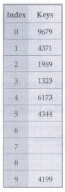
Ex. 7.4.3: Give the input {4371, 1323, 6173, 4199, 4344, 9679, 1989} and hash function X(mod 10), show the results for the following:

i) Open addressing hash table using linear probing

ii) Open addressing hash table using quadratic probing

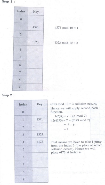
iii)Open addressing hash table with second hash function h² (X) = 7 - (X mod 7).

Sol. i) Open addressing hash table using linear probing :

We assume mod function as mod 10.

4371 mod 10 = 1

1323 mod 10 = 3

6173 mod 10 = 3 collision occurs

Hence by linear probing we will place 6173 at next empty location. That is, at location 4.

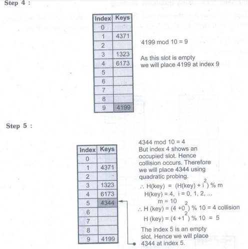
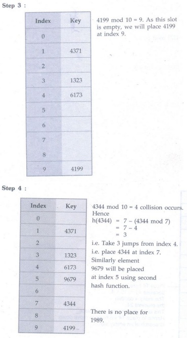
4199 mod 10 = 9

4344 mod 10 = 4 but location 4 is not empty.

Hence we will place 4344 at next empty location i.e. 5,

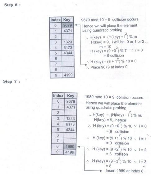
9679 mod 10 = 9 collision occurs so place at next location at 0. The hash table is of size 10. Hence we find the next empty location by rolling the table in forward direction.

1989 mod 10 = 9 collision occurs, so we find the next empty location at index 2.

The hash table will then be

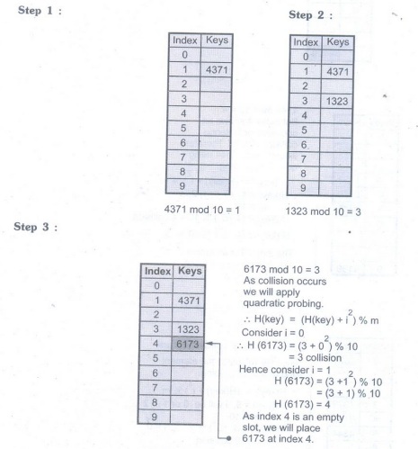
ii) Open addressing hash table using quadratic probing

In quadratic probing we consider the original hash key and then add an arbitrary polynomial. This sum is then considered for hash function. The hash function will be

H(Key)=(Key+i²)% m

where m can be a table size

If we assume m = 10, then the numbers can be inserted as follows

iii) Open addressing hash table with second hash function

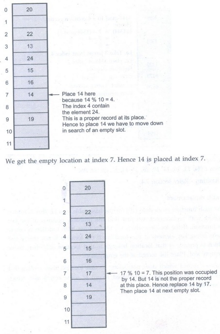
Ex. 7.4.4 : What do you understand by collision in hashing? Represent the following keys in memory using linear probing with or without replacement. Use modulo (10) as your hashing function: (24, 13, 16, 15, 19, 20, 22, 14, 17, 26, 84, 96)

Sol. Collision in hashing - Refer section 7.4.

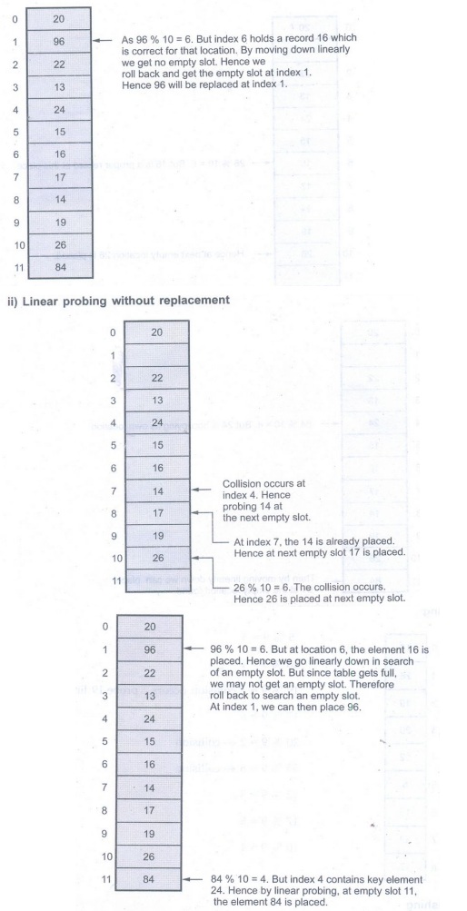
i) Linear probing with replacement

We will consider the hash function as modulo (10) for the hash table size 12, that is from 0 to 11. In linear probing with replacement, we first find the probable position of the key element using hash function. If the location which we obtain from hash function is empty then place the corresponding key element at that location. If the location is not empty and the key element which is present at that location belongs to that location only then, move down in search of empty slot. Place the record at the empty slot.

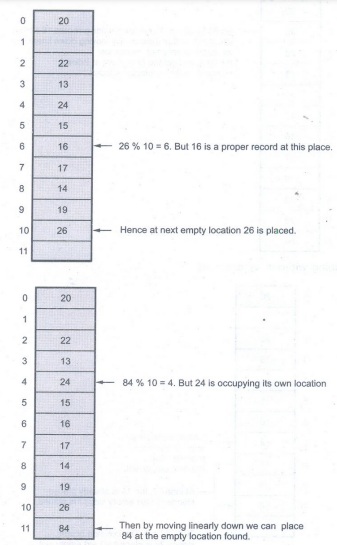
If the location contains a record which does not belong to that location then replace that record by the current key element. Place the replaced record at some empty slot, which can be obtained by moving linearly down.

Ex. 7.4.5 Consider a hash table with 9 slots. The hash function is h(k) = k mod 9. The following keys are inserted in the order 5, 28, 19, 15, 20, 33, 12, 17, 10. Draw the contents of the hash table when the collisions are resolved by

(i) Chaining (ii) Linear probing (iii) Double hashing.

The second hash function h2(x)=7-(x mod 7).

Sol. i) Chaining

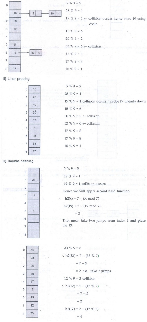
That mean take two jumps from index 1 and place the 19.Similarly remaining elements can be placed. When collision occurs, double hashing is applied.

Rehashing

Rehashing is a technique in which the table is resized, i.e., the size of table is doubled by creating a new table. It is preferable if the total size of table is a prime number. There are situations in which the rehashing is required -

• When table is completely full.

•With quadratic probing when

• When insertions fail due to overflow.

In such situations, we have to transfer entries from old table to the new table by recomputing their positions using suitable hash functions.

Consider we have to insert the elements 37, 90, 55, 22, 17, 49 and 87. The table size is 10 and will use hash function,

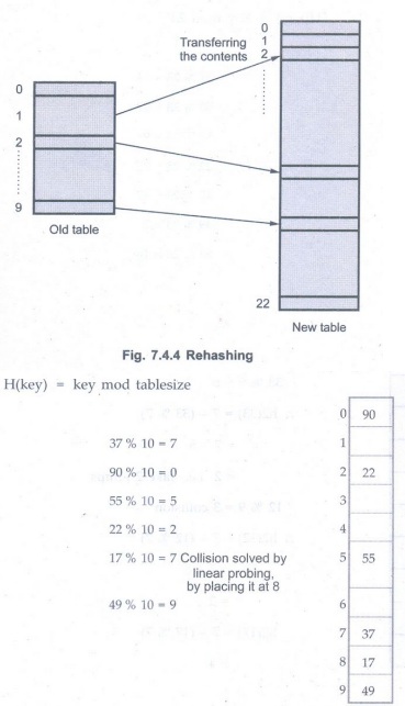
Now this table is almost full and if we try to insert more elements collisions will occur and eventually further insertions will fail. Hence we will rehash by doubling the table size. The old table size is 10 then we should double this size for new table, that becomes 20. But 20 is not a prime number, we will prefer to make the table size as 23. And new hash function will be

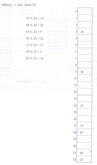
Now the hash table is sufficiently large to accommodate new insertions.

Advantages

1. This technique provides the programmer a flexibility to enlarge the table size if is required. besig in einspaloandfo

2. Only the space gets doubled with simple hash function which avoids occurrence of collisions.

Extendible Hashing

• Extendible hashing is a technique which is useful in handling large amount of data.

• It is one form of dynamic hashing because data are frequently inserted and due to which the hash table size gets changed quite often.

• The data to be placed in the hash table is by extracting certain number of bits.

• The extendible hash table grow and shrink similar to B-trees.

• The extendible hashing scheme contains main memory (Directory) and one or more buckets stored on disk.

• The hash table size is always 2d where d is called global depth. Each table entry points to one bucket.

• Each bucket is associated with local depth d'.

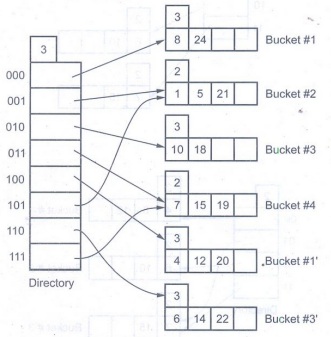
For example

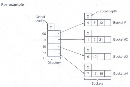
Here binary representation of 4, 8 and 12 is

4 = 0100        8 = 1000          12=1100

The last two bits are 00, hence we will place them in Bucket # 1, because the 00 index of main directory points to Bucket #1. Similarly other elements are placed in appropriate bucket based on last 2 bits. For the sake of understanding, the list of binary representation of the numbers used above is as follows -

1 = 0001, 10 = 1010,

5 = 0101, 7 = 0111,

21 = 10101, 15 = 1111,

6 = 0110, 19 = 10011

Insertion operation

Step 1: If the target bucket does not overflow, simply insert data in appropriate bucket based on bit extract.

Step 2: If bucket overflow happens, then if local depth is equal to global depth and if the d bits are not enough to distingusih the search values of overflown bucket, then directory gets doubled.

Step 3: If local depth is less than the global depth and if bucket gets overflow, then there is no need to double the size of the directory.

For example - Consider following hash table and insert 14, 20, 24, 18, 22

Step 2: Insert 20

Binary representation of 20 = 10100

Insert it in Bucket #1

Step 3: Insert 24 on erity

Binary representation of 24 = 11000

If we insert 24 in Bucket #1, then overflow will occur. As local depth d' of Bucket #1 Global depth d 2. We need to double the size of main directory. Then increment the global depth. Rehash Bucket #1 to place the elements. Note that while rehashing for Bucket #1 elements, last 3 bits are considered. Then update local depth of Bucket #1 and the Bucket that gets created as split image of Bucket #1.

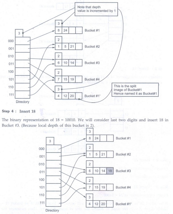
Step 5: Insert 22

The binary representation of 22 = 10110. That means in 22 in Bucket #3. But as Bucket #3 is full we need to create split image of Bucket #3 as Bucket #3'. There is no need to double the size of directory as global depth (3) > local depth (2) of Bucket #3. Now to rehash the values in Bucket #3 and Bucket #3' we will consider last three bits. The local depth of Bucket #3=- Bucket #3'=3. Thus 22 gets inserted appropriately.

Thus insertions can be made in extendible hashing.

Points to Remember :

• The maximum number of bits needed to tell which bucket an entry belongs to for Directory is called global depth.

• The number of bits used to determine if an entry belongs to particular which bucket is called local depth.

•The directory gets doubled only when bucket is full and local depth before insertion.

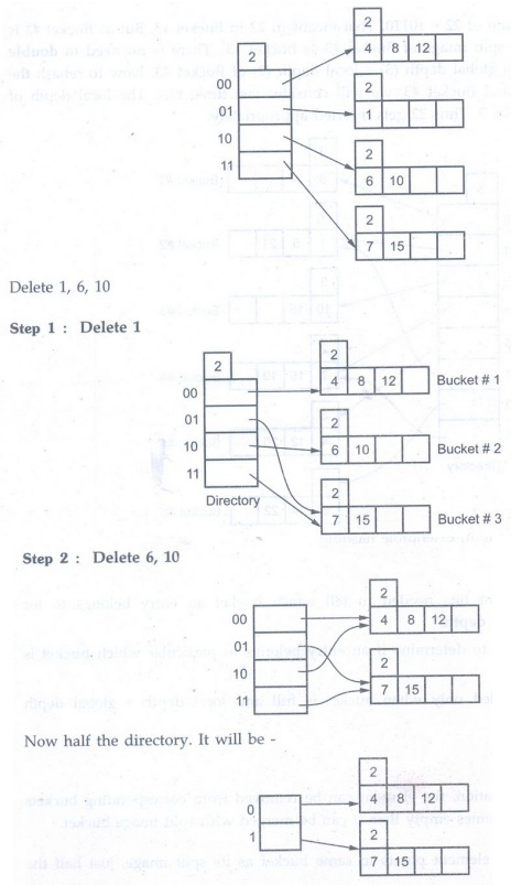
Deletion operation

Step 1: For deletion operation, the element can be removed from corresponding buckets and if bucket becomes empty then it can be merged with split image bucket.

Step 2: If each directory element points to same bucket as its split image, just half the directory.

For example: Consider following hash table

Advantages:

1. The performance of extendible hashing does not get degraded with the growing file size.

2. It requires minimum space overhead.

Disadvantages

1.It contains extra level of indirection for bucket address.

2.This method is complex to implement.

Review Questions

1. Explain the following collision resolution strategies with example.

i) Separate chaining ii) Linear probing iii) Quadratic probing

2. Explain the following: Rehashing.

3. Illustrate with example the open addressing and chaining methods of collision resolution techniques in hashing.

4. Explain open addressing in detail.

6. When do you perform rehashing? Illustrate with example.

5. Explain rehashing and extendible hashing.