Bayesian Learning and Inferencing

Bayesian Learning and Inferencing

AU May-14, Dec.-14

1) It calculates the probability of each hypotheses, given the data and makes the predictions on that basis.

2) Predictions are made by using all the hypotheses, weighted by their probabilities, bay rather than a single "best" hypothesis. This way learning is reduced to probabilistic inference.

3) Let D represent all the data with observed value d, then the probability of each hypothesis obtained by Bayes' Rule -

P(h_i | d) = α P(d | h_i) P(h_j)                                              …….(7.2.1)

If we want to make predicition about an unknown quantity X, then we have, P(X | P(X | d) = Σ_i P(X | d, h_i) P(h_i | d)

= Σ_i P(X | h_i) P (h_i | d)                                        ... (7.2.2)

Where it is assumed that each hypothesis determines a probability distribution over X.

4) Equation (7.2.2) shows that predictions are weighted averages over the predictions of the individual hypotheses.

5) The important quantities in Bayesian learning are the hypothesis prior - P(h_i) and or the likelihood of the data under each hypothesis - P(d | h_i).

6) The basic characteristic of Baysian learning is that "True hypothesis dominates the Bayesian prediction".

7) For any fixed prior that does not rule out the true hypothesis, the posterior probability of any false hypothesis will eventually vanish, simply because the probability of generating "uncharacteristic" data indefinitely is vanishingly small.

8) The Bayesian prediction is optimal whether the data set be small or large.

9) For real learning problems, the hypothesis space is usually very large or infinite.

10) Approximation in Bayesian learning: -

i) A prediction can be made on the basis of single most probable hypothesis, hi, that maximizes P (h_i | d). This is called as maximum a posteriori or MAP hypothesis.

ii) Predictions made according to an MAP hypothesis h map are approximately Bayesian to the extent that P(X | d) ≈ P(X |h_map).

iii) Finding MAP hypothesis is often much easier than Bayesian learning, because it requires solving an optimization problem instead of a large summation.

iv) Overfitting Trade-offs:

  a) Overfitting can occur when the hypothesis space is too expressive, so that it contains many hypotheses that fit the data set well.

  b) Rather than placing an arbitrary limit on the hypotheses to be considered, Bayesian and MAP learning methods use the prior to penalize complexity.

  c) Typically, more complex hypothesis have a lower prior probability-in part because there are usually many more complex hypotheses than simple hypotheses.

  d) On the other hand, more complex hypotheses have a greater capacity to fit the data.

v) Hence, the hypothesis prior embodies a trade-off between the complexity of a (SS) hypothesis and its degree of fit to the data.

vi) If H contains only deterministic hypothesis, then in that case, P(d | h_i) is 1 if h_i is consistent and 0 otherwise. Looking at equation (7.2.1) we see that h_MAP will then be the simplest logical theory that is consistent with the data. Therefore, maximum a posteriori learning provides a natural embodiment of Ockham's razor.

vii) a) Another trade-off between complexity and degree of fit is obtained by taking the logarithm of equation (7.2.1).

b) Choosing h_MAP to maximize P (d | h_i) P(h_i) is equivalent to minimizing

-log₂ P (d | h_i) – log₂ P (h_i)

c) Using the connection between information encoding and probability we see that the -log₂ P(h_i) term equals the number of bits required to specify the hypothesis h_i.

d) log₂ P(d | h_i) is the additional number of bits required to specify the data given the hypothesis.

e) To see this, consider that no bits are required if the hypothesis predicts the data exactly as with h₅ and the string of lime candies and log₂ 1 = 0.

f) MAP learning is choosing the hypothesis that provides maximum compression of the data.

g) The same task is addressed more directly by the minimum description length or MDL, learning method, which attempts to minimize the size of hypothesis and data encodings rather than work with probabilities.

viii) a) Another approximation is provided by assuming a uniform prior over the space of hypotheses. In that case, MAP learning reduces to choosing an h; that maximizes P(d | H_i). This is called a maximum-likelihood (ML) hypothesis, h_ML.

b) Maximum-likelihood learning is very common in statistics, a discipline in which many researchers destruct the subjective nature of hypothesis priors. It is reasonable approach when there is no reason to prefer one hypothesis over another a priori. For example, when all hypotheses are equally complex.

c) It provides a good approximation to Bayesian and MAP learning when the data set is large, because the data swamps the prior distribution over stems hypotheses, but it has problems (all we shall see) with small data sets.

Learning with Complete Data

1. Maximum-Likelihood Parameter Learning: (Discrete Models)

Statistical learning methods have important task which is parameter learning with complete data. Parameter learning task involves finding the numerical parameters for a probability model whose structure is fixed.

Data is said to be complete when each data points contains values for every variable in the mode.

Consider candy-bag example: -

New manufacturer: Then the lime/Cherry proportions is completely unknown.

Parameter: 0 € [0, 1] (proportion of cherry)

Hypothesis: h_Ө

Assumption: All proportions equally likely a priori.

BN's variables: Flavour € {Cherry, Lime}

N unwrapped candies: C cherries and I = N – C limes.

Likelihood of this particular data set:

P(d | h_Ө)=II^N_j=1 P(d_i | |h_Ө) = Ө^c (1 - Ө)ⁱ

• Finding the maximum-likelihood hypothesis h_ML is then equivalent to maximising the log-likelihood:

L(d | h_Ө) = log P(d | h_Ө)

= Σ^N_j=1 log P(d_j | h_Ө) = clog_Ө + l log (1 - Ө)

To that end : 1) differentiate L with respect to 0 and

2) set the resulting expression to 0.

dL(d|h_Ө)/dӨ = c/Ө = l /1- Ө = 0 → Ө = c / c+l = c/N

• Previous result is obvious, but the process is important: -

1) Write down the expression for the likelihood of the data as a function of the parameter(s).

2) Write down the derivative of the log-likelihood with respect to each parameter.

3) Find the parameter values such that the derivatives are zero.

The last step can be tricky, using iterative solution algorithms or numerical optimisation.

Problem with ML learning:

If some events have never been observed, h_ML assigns them 0 probability.

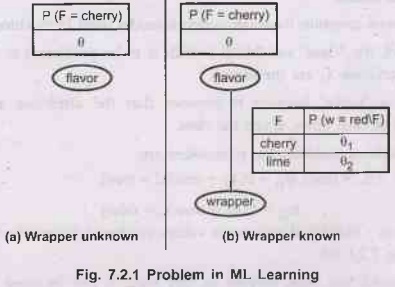
New pb(b): Wrappers red or blue. Colors selected probabilistically (see new BN)

P (Flavor = Cherry, Wrapper = green | h_0,01,02)

= P (Flavor = cherry | h_{Ө, Ө1, Ө2}) P (Wrapper = green | Flavor = Cherry, h_{Ө, Ө1, Ө2})

= Ө. (1- Ө₁)

Experiment:

N = c + l = (r_c + g_c) + (r_l + g_l)

Likelihood:

P(d | h _{Ө, Ө1, Ө2}) = Ө^c (1 - Ө)^l. Ө₁^rc (1 – Ө₁)^gc . Ө₂^r1 (1 – Ө₂)^g1

log-likelihood:

L = [clog Ө + llog (1- Ө)] + [r_c log Ө ₁+ g_c log (1- Ө ₁)]+ [r_l log Ө₂ + g_l log (1- Ө ₂)]

Derivatives:

dL/dӨ = c/Ө – l/1- Ө = 0   => Ө = c/c+l

dL/dӨ₁ = r_c /Ө₁ – g_c /1- Ө₁ = 0   => Ө = r_c /r_c + g_c

dL/dӨ₂ = r_l /Ө₂ – g_l /1- Ө₂ = 0   => Ө = r_l /r_l + g_l

With complete data, ML parameter learning for a BN decomposes into separate learning problems (one per parameter).

2. Naive Bayes Models

1) This is the most common Bayesian network model used in machine learning.

2) In this model, the "class" variable C (which is to be predicted) is the root and the "attribute" variables X_i are the leaves.

3) The model is "naive" because it assumes that the attributes are conditionally independent of each other, given the class.

4) Assuming Boolean variables the parameters are,

Ꮎ = P(C = true), Ꮎ_i1 =P(X_i = true | C = true),

Ꮎ_i2 = P(X_i= true | C = false)

The maximum likelihood parameter values are found in exactly the same way as shown in Fig. 7.2.1 (b).

5) Once the model has been trained in this way, it can be used to classify new examples for which the class variable C is unobserved. With observed attribute values, x₁, x₂,.... x_n, the probability of each class is given by,

P(C x₁, x₂,… x_n) = α P(C) II_i P(x_i | C)

6) A deterministic prediction can be obtained by choosing the most likely class.

7) The method learns fairly well but not as well as decision-tree learning; this is presumably because the true hypothesis which is a decision tree is not representable exactly using a naive Bayes model.

8) Naive Bayes learning do well in a wide range of applications; the boosted version is one of the most effective general-purpose learning algorithm.

9) Naive Bayes learning scales well to very large problems with n Boolean attributes, there are just 2n+1 parameters, and no search is required to find h_ML, the maximum likelihood naive Bayes hypothesis.

10) Naive Bayes learning has no difficulty with noisy data and can give probabilistic predictions when appropriate.

3. Maximum-Likelihood Parameter Learning (Continuous Models)

1) Continuous probability model such as the linear-Gaussian model is used for maximum - likelihood parameter learning.

2) Because continuous variables are ubiquitous in real-world applications, it is important to know how to learn continuous models from data.

3) The principles for maximum likelihood learning are identical to those of the discrete case.

4) a) Let us begin with a very simple case: Learning the parametes of a Gaussian density function on a single variable.

b) That is, the data are generated as follows: -

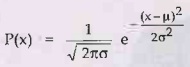
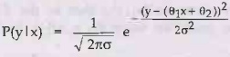
The parameters of this model are the mean u and the standard deviation σ. (Notice that the normalizing "constant" depends on σ, so we cannot ignore it.

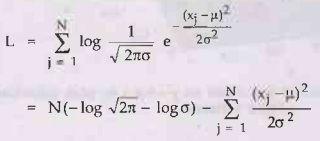
c) Let the observed values be x₁,..., x_N. Then the log likelihood is,

d) Setting the derivatives to zero as usual, we obtain,

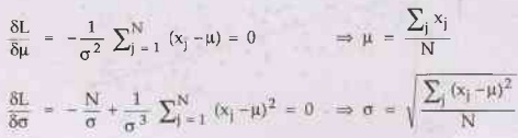
5) The maximum-likelihood value of the mean is the sample average and the maximum-likelihood value of the standard deviation is the square root of the sample variance. Again, these are comforting results that confirm "commonsense" practice.

6) a) Now consider a linear Gaussian model with one continuous parent X and acontinuous child Y.

b) Y has a Gaussian distribution whose mean depends linearly on the value of X and whose standard deviation is fixed.

c) To learn the conditional distribution P(Y|X), we can maximize the conditional likelihood.

d) Here, the parameters are Ө₁, Ө₂ and σ. The data are a collection of (x_j, y_j)

pairs, as shown in Fig. 7.2.4.

e) Using the usual methods, we can find the maximum-likelihood values of theparameters.

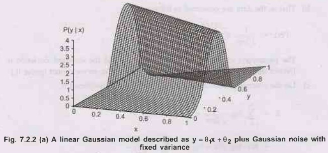
f) Here we want to make a different point. If we consider just the parameters Ө₁ and Ө₂ that define the linear relationship between x and y, it becomes clear that maximizing the log-likelihood with respect to these parameters is the same as minimizing the numerator in the exponent of above equation.

E =Σ^N_j=1 ( y_j - (Ѳ₁ x_j +Ѳ₂)²

g) The quantity (y_j -(Ѳ₁ x_j +Ѳ₂)) is the error for (x_j, y_j) that is, the difference between the actual value y_i and the predicted value (Ѳ₁ x_j + Ѳ₂). So E is the well-known sum of squared errors.

(h) This is the quantity that is minimized by the standard linear regression procedure.

i) Minimizing the sum of squared errors gives the maximum - likelihood straight line model, provided that the data are generated with Gaussian noise of fixed variance.

4. Bayesian Parameter Learning

ML learning is simple, but not appropriate for small data sets.

Example -

If only cherries have been observed, h_ML →0=1.0

• Bayesian Approach:

  - It uses hypothesis prior over possible values of the parameters.

  - Update of this distribution is used as the data arrives.

• Candy example with Bayesian view :-

  - Ө unknown value of a variable Ѳ.

  - Hypothesis prior: P (Ѳ). (Continuous over [0, 1] and integrating to 1).

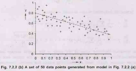
• Candidates:

beta distributions, defined by 2 hyperparameters a and b

such that:

beta [a, b] (Ѳ) = αѲ^a-1 (1-Ѳ)^b-1

• Nice property of the beta family:

If Ѳ has prior beta [a, b] and a data point is observed, then the posterior for is also a beta distribution.

Beta family:

A beta family is called as the conjugate prior for the family of distributions for a

Boolean variable.

P(Ѳ | D1 Cherry)=α P(D₁=Cherry | Ѳ) P(Ѳ)

= α՛ Ѳ. Beta[a,b] (Ѳ) = α՛ Ѳ. Ѳ^a-1 (1- Ѳ)^b-1

= α՛ Ѳ^a (1- Ѳ)^b-1 = beta [a + 1, b] (Ѳ)

Note: a and b are virtual counts (starting with beta [1, 1]).

With wrappers: 3 parameters. It need to specify P(Ѳ, Ѳ_1, Ѳ₂).

Assuming parameter independence: P (Ѳ, Ѳ_1, Ѳ₂) = P(Ѳ) P (Ѳ₁) P (Ѳ₂)

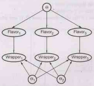
Fig. 7.2.4 A Bayesian network that corresponds to a Bayesian learning process. Posterior distributions for the parameter variables 0, 1, 2 can be inferred from their prior distributions and the evidence in the flavour, wrapper; variables

• View of Bayesian learning as inference in a BN.

Variables: Unknown parameters + variables describing each instance.

P (Flavor_i= Cherry | Ѳ = Ө) = Ө

P (Wrapper_i = red | Flavor_i = Cherry, Ѳ₁ = Ө₁) = Ө₁

5. Learning Bayes Net Structures

Often the Bayes net structures are easy to get from expert knowledge. But sometimes the causality relationships are debatable.

For example:

Smoking => Cancer?

too Much TV => Bad at school?

• To search for a good model:

- Start with a linkless model and add parents to each node, then learn parameters and measure accuracy of the resulting model.

- Start with an initial guess of the structure, and use hill-climbing or simulated annealing to make modifications (reversing, adding, or deleting arcs).

Note

• Two ways for deciding when a good structure has been found: -

1) Test whether the conditional independence assertions implicit in the structure, are satisfied in the data.

P(Fri Sat, Bar | WillWait)=P(Fri Sat WillWait) P(Bar | WillWait)

It requires an appropriate statistical test (with appropriate threshold).

2) Measure the degree to which the proposed model explains the data. The ML hypothesis would give a fully connected network.

• Here we need to penalize complexity: -

a) MAP (MDL) approach: Substracts a penalty from the likelihood of each structure.

b) Bayesian approach: places a joint prior over structures and parameters.

It too many structures are there then use sampling rather than exact methods.