Algorithms for Selection,Sorting and Join Operations

Algorithms for Selection, Sorting and join Operations

AU: Dec.-19, Marks 3

Algorithm for Selection Operation

For selection operation, the file scan is an important activity. Basically file scan is a based on searching algorithms. These searching algorithms locate and retrieve the records that fulfills a selection condition.

Let us discuss various algorithms used for SELECT Operation based in file scan 

Algorithm A1: Linear Search

• Scan each file block and test all records to see whether they satisfy the selection condition

Cost - b_r block transfers + 1 seek

Where,

b_r denotes number of blocks containing records from relation r

• If selection is on a key attribute, can stop on finding record

Cost = (br/2) block transfers + 1 seek

• Advantages of Linear Search

 • Linear search works even-if there is no selection condition specified.

 • For linear search, there is no need to have records in the file in ordered form.

 • Linear search works regardless of indices.

Algorithm A2: Binary Search

• Applicable if selection is an equality comparison on the attribute on which file is ordered.

• Assume that the blocks of a relation are stored contiguously.

• Cost estimate is nothing but the number of disk blocks to be scanned.

• Cost of locating the first tuple by a binary search on the blocks = [log₂(b_r)] x (t_T + t_S) Where,

b_r denotes number of blocks containing records from relation r

t_T is average time required to transfer a block of data, in seconds

t_S is average block access time, in second

• If there are multiple records satisfying the selection add transfer cost of the number of blocks containing records that satisfy selection condition.

Algorithm for Sorting Operation

External sorting

• In external sorting, the data stored on secondary memory is part by part loaded into main memory, sorting can be done over there.

• The sorted data can be then stored in the intermediate files. Finally these intermediate files can be merged repeatedly to get sorted data.

• Thus huge amount of data can be sorted using this technique.

• The external merge sort is a technique in which the data is loaded in intermediate files. Each intermediate file is sorted independently and then combined or merged to get the sorted data. 

For example : Consider that there are 10,000 records that has to be sorted. Clearly we need to apply external sorting method. Suppose main memory has a capacity to store 500 records in blocks, with each block size of 100 records

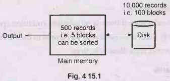
The sorted 5 blocks (i.e. 500 records) are stored in intermediate file. This process will be repeated 20 times to get all the records sorted in chunks.

In the second step, we start merging a pair of intermediate files in the main memory to get output file.

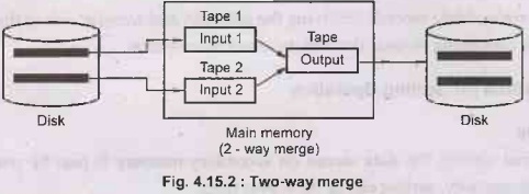
Multiway merge

• Multiway merge sort is a technique of merging 'm' sorted lists into single sorted list. The two-way merge is a special case of multiway merge sort.

Let us understand it with the help of an example.

Example 4.15.1 Sort the following list of elements using two way merge sort with M = 3. 20, 47, 15, 8, 9, 4, 40, 30, 12, 17, 11, 56, 28, 35.

Solution: As M = 3, we will break the records in the group of 3 and sort them. Then we will store them on tape. We will store data on alternate tapes.

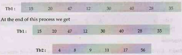
Stage I: Sorting phase

1) 20, 47, 15. We arrange in sorted order → 15, 20, 47

2) Read next three records sort them and store them on Tape Tb2

8,9,4→4,8,9

3) Read next three records, sort them and store on tape Tb1.

40,30,12→12,30,40

4) Read next three records, sort them and store on tape Tb2.

17, 11, 56→11, 17, 56

5) Read next two remaining records, sort them and store on Tape Tb1

28, 35→28, 35

Stage II: Merging of runs

The input tapes Tb1 and Tb2 will use two more output tapes Ta1 and Ta2, for sorting. Finally the sorted data will be on tape Ta1.

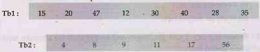
We will read the elements from both the tapes Tb1 and Tb2, compare them and store on Ta1 in sorted order.

Now we will read second blocks from Tb1 and Tb2. Sort the elements and store on Ta2.

Finally read the third block from Tb1 and store in sorted manner on Tal. We will not compare this block with Ta2 as there is no third block. Hence we will get

Now compare first blocks of Tal and Ta2 and store sorted elements on Tb1.

Now both Tb1 and Tb2 contains only single block each. Sort the elements from both the blocks and store the result on Ta1.

Thus we get sorted list.

Algorithm

Step 1: Divide the elements into the blocks of size M. Sort each block and write runs on disk.

Step 2: Merge two runs

i) Read first value on each of two runs

ii) Compare and sort

iii) Write on output tape.

Step 3: Repeat the step 2 and get longer and longer runs on alternate tapes. Finally we will get single sorted list.

Analysis: The algorithm requires log(N/M) Passes plus initial run construction pass.

• Initially

1st tape contains N records = M records * N/M runs.

After storing the runs on two tapes, each contains half of the runs

Two tapes * M_records per run*1/2 (N/M) = = N records

• After merge 1st pass - double the length of runs, halve the number of runs

Two tapes *2M_records run *1/2*1/2= (N,M) per runs = N records

• After merge 2nd,pass

Two tapes 4 M_records per run *1/2*1/2 *(N,M) runs = N records

• After merge S-th pass

Two tapes * 2^S M records per run *(1/2^s) (1/2) (N/M) runs = N records

• After the last merge, there will be only one run equal to whole file.

2^S M = N

2^S  = N/M

S= log (N/M)

Hence at each pass the N records are processed and we get the time complexity as O (N log (N/M)).

• The two way merge sort makes use of two input tapes and two output tapes for sorting the records.

• It works in two stages -

Stage 1: Break the records into block. Sort individual record with the help of two input tapes.

Stage 2: Merge the sorted blocks and create a single sorted file with the help of two output tapes.

Algorithm for Join Operation

• JOIN operation is the most time consuming operation to process.

• There are Several different algorithms to implement joins

1. Nested-loop join

2. Block nested-loop join

3. Indexed nested- loop join

4. Merge-join

5. Hash-join

Choice of a particular algorithm is based on cost estimate.

Algorithm For Nested Loop Join

This algorithm is for computing r  Ө s

Let, r is called the outer relation and s the inner relation of the join. A

for each tuplet t_r in r do begin

for each tuple t_s in s do begin

test pair (t_r,t_s) to see if they satisfy the join condition

if 0 is satisfied, then, add (t_r, t_s) to the result,

end

end

• This algorithm requires no indices and can be used with any kind of join condition.

• It is expensive since it examines every pair of tuples in the two relations.

• In the worst case, if there is enough memory only to hold one block of each relation, the estimated cost is

• n_r × b_s + b_r block transfers, plus n_r + b_r seeks

• If the smaller relation fits entirely in memory, use that as the inner relation

   • Reduces cost to b_r + b_s block transfers and 2 seeks

• For example Assume the query CUSTOMERS  ORDERS (with join attribute only being CName)

Number of records of customer: 10000 order: 5000

Number of blocks of customer: 400 order: 100

Formula Used:

(1) n_r × b_s + b_r block transfers,

(2) n_r + b_r seeks

r is outer relation and s is inner relation.

With order as outer relation:

n_r= 5000 b_s= 400, b_r = 100

5000 × 400 + 100 = 2000100 block transfers and

5000+100 5100 seeks

With customer as the outer relation :

n_r =10000, b_s =100, b_r =400

10000 x 100 + 400 = 1000400 block transfers and

10000+400=10400 seeks

If smaller relation (order) fits entirely in memory, the cost estimate will be: 

b_r+b_s =500 block transfers

Algorithm For Block Nested Loop Join

Variant of nested-loop join in which every block of inner relation is paired with every block of outer relation.

This algorithm is for computing r Ө s

Let, r is called the outer relation and s the inner relation of the join.

for each block B_r of r do

for each block B_s of s do

for each tuple t_r in B_r do begin

for each tuple t_s in B_s do begin

test pair (t_r, t_s) to see if they satisfy the join condition

if Ө is satisfied, then, add (t_r, t_s) to the result.

end

end

end

end

Worst case estimate: b_r × b_s + b_r block transfers + 2 × b_r seeks

Each block in the inner relation s is read once for each block in the outer relation. Best case: b_r+ b_s block transfers + 2 seeks

(3) Merge Join

• In this operation, both the relations are sorted on their join attributes. Then merged these sorted relations to join them.

• Only equijoin and natural joins are used.

• The cost of merge join is,

b_r + b_s block transfers + [b_r /b_b] + [b_s/b_b] seeks + the cost of sorting, if relations are unsorted.

(4) Hash Join

• In this operation, the hash function h is used to partition tuples of both the relations.

• h maps A values to {0, 1, ..., n}, where A denotes the attributes of r and s used in the join.

• Cost of hash join is:

3(b_r+b_s) + 4 x n block transfers + 2([b_r /b_b] + [b_s/b_b]) seeks

If the entire build input can be kept in main memory no partitioning is required Cost estimate goes down to br+bs.

Review Question

1. With simple example explain the computing of Nested loop-join and block nested loop join. AU: Dec.-19, Marks 3